Inverse Problems
In traditional imaging, the burden of image formation is placed on physical components, such as a lens, with the resulting image being taken from the sensor with minimal processing. In computational imaging, in contrast, the burden of image formation is shared with or shifted to computation, with the resulting image typically being very different from the measured data. Common examples of computational imaging include demosaicing in consumer cameras, computed tomography and magnetic resonance imaging in medicine, and synthetic aperture radar in remote sensing. This is an active and growing area of research, and many of these problems have common properties that could be supported by shared implementations of solution components.
The goal of SCICO is to provide a general research tool for computational imaging, with a particular focus on scientific imaging applications, which are particularly underrepresented in the existing range of open-source packages in this area. While a number of other packages overlap somewhat in functionality with SCICO, only a few support execution of the same code on both CPU and GPU devices, and we are not aware of any that support just-in-time compilation and automatic gradient computation, which is invaluable in computational imaging. SCICO provides all three of these valuable features (subject to some caveats) by being built on top of JAX rather than NumPy.
The remainder of this section outlines the steps involved in solving an inverse problem, and shows how each concept maps to a component of SCICO. More detail on the main classes involved in setting up and solving an inverse problem can be found in Main SCICO Classes.
Forward Modeling
In order to solve a computational imaging problem we need to know how the image we wish to reconstruct, \(\mathbf{x}\), is related to the data that we can measure, \(\mathbf{y}\). This is represented via a model of the measurement process,
SCICO provides the Operator and LinearOperator
classes, which may be subclassed by users, in order to implement the
forward operator, \(A\). It also has several built-in operators,
most of which are linear, e.g., finite convolutions, discrete Fourier
transforms, optical propagators, Abel transforms, and X-ray transforms
(the same as Radon transforms in 2D). For example,
input_shape = (512, 512)
angles = np.linspace(0, 2 * np.pi, 180, endpoint=False)
channels = 512
A = scico.linop.xray.svmbir.XRayTransform(input_shape, angles, channels)
defines a tomographic projection operator.
A significant advantage of SCICO being built on top of JAX is that the adjoints of
linear operators, which can be quite time consuming to implement even
when the operator itself is straightforward, are computed
automatically by exploiting the automatic differentation features of
JAX. If A is a
LinearOperator, then its adjoint is simply A.T for
real transforms and A.H for complex transforms. Likewise,
Jacobian-vector products can be automatically computed for non-linear
operators, allowing for simple linearization and gradient
calculations.
SCICO operators can be composed to construct new operators. (If both
operands are linear, then the result is also linear.) For example, if
A and B have been defined as distinct linear
operators, then
C = B @ A
defines a new linear operator C that first applies operator
A and then applies operator B to the result
(i.e. \(C = B A\) in math notation). This operator algebra can be
used to build complicated forward operators from simpler building
blocks.
SCICO also handles cases where either the image we want to
reconstruct, \(\mb{x}\), or its measurements, \(\mb{y}\), do
not fit neatly into a multi-dimensional array. This is achieved via
BlockArray objects, which consist of a list of
multi-dimensional array blocks. A BlockArray differs from
a list in that, whenever possible, BlockArray
properties and methods (including unary and binary operators like
+, -, *, …) automatically map along the blocks, returning
another BlockArray or tuple as appropriate. For
example, consider a system that measures the column sums and row sums
of an image. If the input image has shape \(M \times N\), the
resulting measurement will have shape \(M + N\), which is awkward
to represent as a multi-dimensional array. In SCICO, we can represent
this operator by
input_shape = (130, 50)
H0 = scico.linop.Sum(input_shape, axis=0)
H1 = scico.linop.Sum(input_shape, axis=1)
H = scico.linop.VerticalStack((H0, H1))
The result of applying H to an image with shape (130, 50) is a
BlockArray with shape ((50,), (130,)). This result is
compatible with the rest of SCICO and may be used, e.g., as the input
of other operators.
Inverse Problem Formulation
In order to estimate the image from the measured data, we need to solve an inverse problem. In its simplest form, the solution to such an inverse problem can be expressed as the optimization problem
where \(\mb{x}\) is the unknown image and \(\hat{\mb{x}}\) is the recovered image. A common choice of \(f\) is
where \(\mb{y}\) is the measured data and \(A\) is the forward operator; in this case the minimization problem is a least squares problem.
In SCICO, the functional module provides implementations of common
functionals such as \(\ell_2\) and \(\ell_1\) norms. The
loss module is used to implement a special type of functional
where \(\alpha\) is a scaling parameter and \(l(\cdot)\) is
another functional. The SCICO loss module contains a variety
of loss functionals that are commonly used in computational
imaging. For example, the squared \(\ell_2\) loss written above
for a forward operator, \(A\), can be defined in SCICO using the
code:
f = scico.loss.SquaredL2Loss(y=y, A=A)
The difficulty of the inverse problem depends on the amount of noise in the measured data and the properties of the forward operator. In particular, if \(A\) is a linear operator, then the difficulty of the inverse problem depends significantly on the condition number of \(A\), since a large condition number implies that large changes in \(\mb{x}\) can correspond to small changes in \(\mb{y}\), making it difficult to estimate \(\mb{x}\) from \(\mb{y}\). When there is a significant amount of measurement noise or ill-conditioning of \(A\), the standard approach to resolve the limitations in the information available from the measured data is to introduce a prior model of the solution space, which is typically achieved by adding a regularization term to the data fidelity term, resulting in the optimization problem
where the functional \(g(C(\cdot))\) is designed to increase the cost for solutions that are considered less likely or desirable, based on prior knowledge of the properties of the solution space. A common choice of \(g(C(\cdot))\) is the total variation norm
where \(\lambda\) is a scalar controlling the regularization
strength, \(C\) is a linear operator that computes the spatial
gradients of its argument, and \(\| \cdot \|_{2,1}\) denotes the
\(\ell_{2,1}\) norm, which promotes group sparsity. Use of this
functional as a regularization term corresponds to the assumption that
the images of interest are piecewise constant. In SCICO, we can
represent this regularization functional using a built-in linear
operator and a member of the functional module:
C = scico.linop.FiniteDifference(A.input_shape, append=0)
λ = 1.0e-1
g = λ * scico.functional.L21Norm()
Computing the value of the regularizer then closely matches the math:
g(C(x)).
Finally, the overall objective function needs to be optimized. One of the primary goals of SCICO is to make the solution of such problems accessible to application domain scientists with limited expertise in computational imaging, providing infrastructure for solving this type of problem efficiently, without the need for the user to implement complex algorithms.
Solvers
Once an inverse problem has been specified using the above components, the resulting functional must be minimized in order to solve the problem. SCICO provides a number of optimization algorithms for addressing a wide range of problems. These optimization algorithms belong to two distinct categories.
Basic Solvers
The scico.solver module provides a number of functions for
solving linear systems and simple optimization problems, some of which
are useful as subproblem solvers within the proximal algorithms
described in the following section. It also provides an interface to
functions in scipy.optimize, supporting their use with
multi-dimensional arrays and scico Functional objects. These
algorithms are useful both as subproblem solvers within the proximal
algorithms described below, as well as for direct solution of
higher-level problems.
For example,
f = scico.loss.PoissonLoss(y=y, A=A)
method = 'BFGS' # or any method available for scipy.optimize.minimize
x0 = scico.numpy.ones(A.input_shape)
res = scico.solver.minimize(f, x0=x0, method=method)
x_hat = res.x
defines a Poisson objective function and minimizes it using the BFGS [44] algorithm.
Proximal Algorithms
The scico.optimize sub-package provides a set of proximal
algorithms [47] that have proven to be useful
for solving imaging inverse problems. The common feature of these
algorithms is their exploitation of the proximal operator
[7] (Ch. 6), of the components of the functions
that they minimize.
ADMM The most flexible of the proximal algorithms supported by SCICO is the alternating direction method of multipliers (ADMM) [26] [24] [12], which supports solving problems of the form
When \(f(\cdot)\) is an instance of scico.loss.SquaredL2Loss,
i.e.,
for linear operator \(A\) and constant vector \(\mb{y}\), the primary computational cost of the algorithm is typically in solving a linear system involving a weighted sum of \(A^\top A\) and the \(C_i^\top C_i\), assuming that the proximal operators of the functionals \(g_i(\cdot)\) can be computed efficiently. This linear system can also be solved efficiently when \(A\) and all of the \(C_i\) are either identity operators or circular convolutions.
Proximal ADMM Proximal ADMM [19] solves problems of the form
where \(A\) and \(B\) are linear operators. There is also a non-linear PADMM solver [11] for problems of the form
where \(H\) is a function. For some problems, proximal ADMM converges substantially faster than ADMM or linearized ADMM.
Linearized ADMM Linearized ADMM [61] [47] solves a more restricted problem form,
It is an effective algorithm when the proximal operators of both \(f(\cdot)\) and \(g(\cdot)\) can be computed efficiently, and has the advantage over “standard” ADMM of avoiding the need for solving a linear system involving \(C^\top C\).
PDHG Primal–dual hybrid gradient (PDHG) [22] [14] [48] solves the same form of problem as linearized ADMM
but unlike the linearized ADMM implementation, both linear and non-linear operators \(C\) are supported. For some problems, PDHG converges substantially faster than ADMM or linearized ADMM.
PGM and Accelerated PGM The proximal gradient method (PGM) [18] and accelerated proximal gradient method (APGM), which is also known as FISTA [7], solve problems of the form
where \(f(\cdot)\) is assumed to be differentiable, and \(g(\cdot)\) is assumed to have a proximal operator that can be computed efficiently. These algorithms typically require more iterations for convergence than ADMM, but can provide faster convergence with time when the linear solve required by ADMM is slow to compute.
Machine Learning
While relatively simple regularization terms such as the total variation norm can be effective when the underlying assumptions are well matched to the data (e.g., the reconstructed images for certain materials science applications really are approximately piecewise constant), it is difficult to design mathematically simple regularization terms that adequately represent the properties of the complex data that is often encountered in practice. A widely-used alternative framework for regularizing the solution of imaging inverse problems is plug-and-play priors (PPP) [56] [53] [36], which provides a mechanism for exploiting image denoisers such as BM3D [17] as implicit priors. With the rise of deep learning methods, PPP provided one of the first frameworks for applying machine learning methods to inverse problems via the use of learned denoisers such as DnCNN [64].
SCICO supports PPP inverse problems solutions with both BM3D and DnCNN denoisers, and provides usage examples for both choices. BM3D is more flexible, as it includes a tunable noise level parameter, while SCICO only includes DnCNN models trained at three different noise levels (as in the original DnCNN paper), but DnCNN has a significant speed advantage when GPUs are available. As an example, the following code outline demonstrates a PPP solution, with a non-negativity constraint and a 17-layer DnCNN denoiser as a regularizer, of an inverse problem with measurement, \(\mb{y}\), and a generic linear forward operator, \(A\).
ρ = 0.3  # ADMM penalty parameter
maxiter = 10 # number of ADMM iterations

f = scico.loss.SquaredL2Loss(y=y, A=A)
g1 = scico.functional.DnCNN("17M")
g2 = scico.functional.NonNegativeIndicator()
C = scico.linop.Identity(A.input_shape)

solver = scico.optimize.admm.ADMM(
  f=f,
  g_list=[g1, g2],
  C_list=[C, C],
  rho_list=[ρ, ρ],
  x0=A.T @ y,
  maxiter=maxiter,
  subproblem_solver=scico.optimize.admm.LinearSubproblemSolver(),
  itstat_options={"display": True, "period": 5},
)

x_hat = solver.solve()
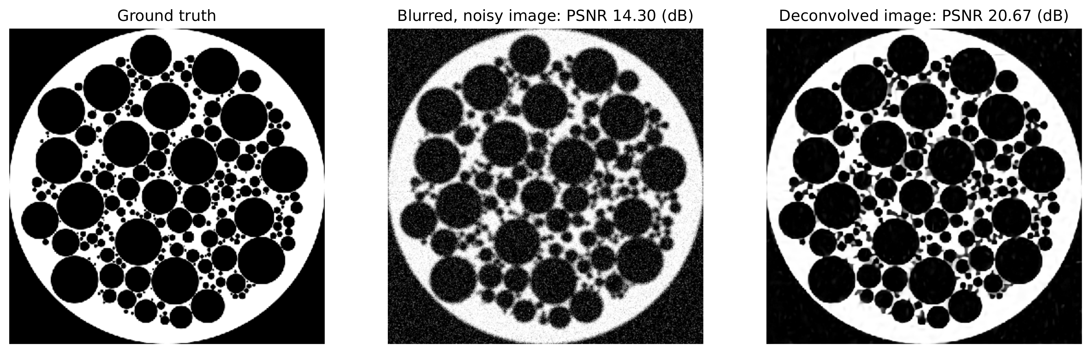
Example results for this type of approach applied to image deconvolution (i.e. with forward operator, \(A\), as a convolution) are shown in the figure below.
More recently, a wider variety of frameworks have been developed for applying deep learning methods to inverse problems, including the application of the adjoint of the forward operator to map the measurement to the solution space followed by an artifact removal CNN [32], and learned networks with structures based on the unrolling of iterative algorithms such as PPP [43]. A number of these methods are currently being implemented, and will be included in a future SCICO release. It is worth noting, however, that while some of these methods offer superior performance to PPP, it is at the cost of having to train the models with problem-specific data, which may be difficult to obtain, while PPP is often able to function well with a denoiser trained on generic image data.