Deconvolution Microscopy (Single Channel)

This example partially replicates a GlobalBioIm example using the microscopy data provided by the EPFL Biomedical Imaging Group.

The deconvolution problem is solved using class admm.ADMM to solve an image deconvolution problem with isotropic total variation (TV) regularization

\[\mathrm{argmin}_{\mathbf{x}} \; (1/2) \| M (\mathbf{y} - A \mathbf{x}) \|_2^2 + \lambda \| C \mathbf{x} \|_{2,1} + \iota_{\mathrm{NN}}(\mathbf{x}) \;,\]

where \(M\) is a mask operator, \(A\) is circular convolution, \(\mathbf{y}\) is the blurred image, \(C\) is a convolutional gradient operator, \(\iota_{\mathrm{NN}}\) is the indicator function of the non-negativity constraint, and \(\mathbf{x}\) is the desired image.

import scico.numpy as snp
from scico import functional, linop, loss, plot, util
from scico.examples import downsample_volume, epfl_deconv_data, tile_volume_slices
from scico.optimize.admm import ADMM, CircularConvolveSolver
plot.config_notebook_plotting()

Get and preprocess data. We downsample the data for the for purposes of the example. Reducing the downsampling rate will make the example slower and more memory-intensive. To run this example on a GPU it may be necessary to set environment variables XLA_PYTHON_CLIENT_ALLOCATOR=platform and XLA_PYTHON_CLIENT_PREALLOCATE=false. If your GPU does not have enough memory, you can try setting the environment variable JAX_PLATFORM_NAME=cpu to run on CPU.

channel = 0
downsampling_rate = 2

y, psf = epfl_deconv_data(channel, verbose=True)
y = downsample_volume(y, downsampling_rate)
psf = downsample_volume(psf, downsampling_rate)

y -= y.min()
y /= y.max()
psf /= psf.sum()

Pad data and create mask.

padding = [[0, p] for p in snp.array(psf.shape) - 1]
y_pad = snp.pad(y, padding)
mask = snp.pad(snp.ones_like(y), padding)

Define problem and algorithm parameters.

λ = 2e-6  # ℓ1 norm regularization parameter
ρ0 = 1e-3  # ADMM penalty parameter for first auxiliary variable
ρ1 = 1e-3  # ADMM penalty parameter for second auxiliary variable
ρ2 = 1e-3  # ADMM penalty parameter for third auxiliary variable
maxiter = 100  # number of ADMM iterations

Create operators.

M = linop.Diagonal(mask)
C0 = linop.CircularConvolve(h=psf, input_shape=mask.shape, h_center=snp.array(psf.shape) / 2 - 0.5)
C1 = linop.FiniteDifference(input_shape=mask.shape, circular=True)
C2 = linop.Identity(mask.shape)

Create functionals.

g0 = loss.SquaredL2Loss(y=y_pad, A=M)  # loss function (forward model)
g1 = λ * functional.L21Norm()  # TV penalty (when applied to gradient)
g2 = functional.NonNegativeIndicator()  # non-negativity constraint

Set up ADMM solver object and solve problem.

solver = ADMM(
    f=None,
    g_list=[g0, g1, g2],
    C_list=[C0, C1, C2],
    rho_list=[ρ0, ρ1, ρ2],
    maxiter=maxiter,
    itstat_options={"display": True, "period": 10},
    x0=y_pad,
    subproblem_solver=CircularConvolveSolver(),
)

print("Solving on %s\n" % util.device_info())
solver.solve()
solve_stats = solver.itstat_object.history(transpose=True)
x_pad = solver.x
x = x_pad[: y.shape[0], : y.shape[1], : y.shape[2]]

Solving on GPU (NVIDIA GeForce RTX 2080 Ti)

Iter  Time      Objective  Prml Rsdl  Dual Rsdl
-----------------------------------------------
   0  1.13e+01  2.830e-01  2.780e+02  1.949e+02
  10  1.86e+01  1.033e+00  5.524e+01  9.689e+01
  20  2.47e+01  1.158e+00  7.474e+01  4.940e+01
  30  3.07e+01  1.297e+00  4.547e+01  5.652e+01
  40  3.66e+01  1.528e+00  4.879e+01  3.606e+01
  50  4.24e+01  1.733e+00  3.740e+01  3.763e+01
  60  4.84e+01  1.919e+00  3.390e+01  3.228e+01
  70  5.45e+01  2.133e+00  2.996e+01  2.785e+01
  80  6.04e+01  2.341e+00  2.456e+01  2.723e+01
  90  6.62e+01  2.560e+00  2.437e+01  2.325e+01
  99  7.16e+01  2.754e+00  2.242e+01  2.143e+01

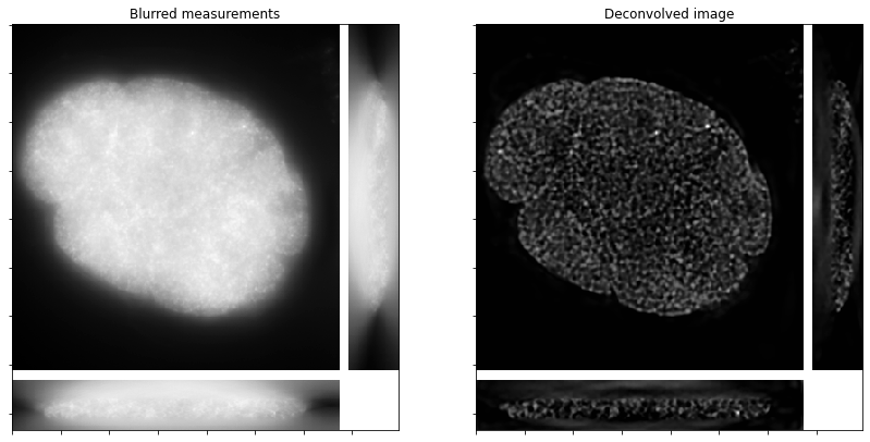
Show the recovered image.

fig, ax = plot.subplots(nrows=1, ncols=2, figsize=(14, 7))
plot.imview(tile_volume_slices(y), title="Blurred measurements", fig=fig, ax=ax[0])
plot.imview(tile_volume_slices(x), title="Deconvolved image", fig=fig, ax=ax[1])
fig.show()

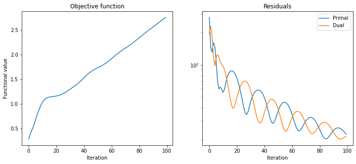
Plot convergence statistics.

fig, ax = plot.subplots(nrows=1, ncols=2, figsize=(12, 5))
plot.plot(
    solve_stats.Objective,
    title="Objective function",
    xlbl="Iteration",
    ylbl="Functional value",
    fig=fig,
    ax=ax[0],
)
plot.plot(
    snp.vstack((solve_stats.Prml_Rsdl, solve_stats.Dual_Rsdl)).T,
    ptyp="semilogy",
    title="Residuals",
    xlbl="Iteration",
    lgnd=("Primal", "Dual"),
    fig=fig,
    ax=ax[1],
)
fig.show()