Complex Total Variation Denoising with PDHG Solver
This example demonstrates solution of a problem of the form
where \(C\) is a nonlinear operator, via non-linear PDHG [55]. The example problem represents total variation (TV) denoising applied to a complex image with piece-wise smooth magnitude and non-smooth phase. The appropriate TV denoising formulation for this problem is
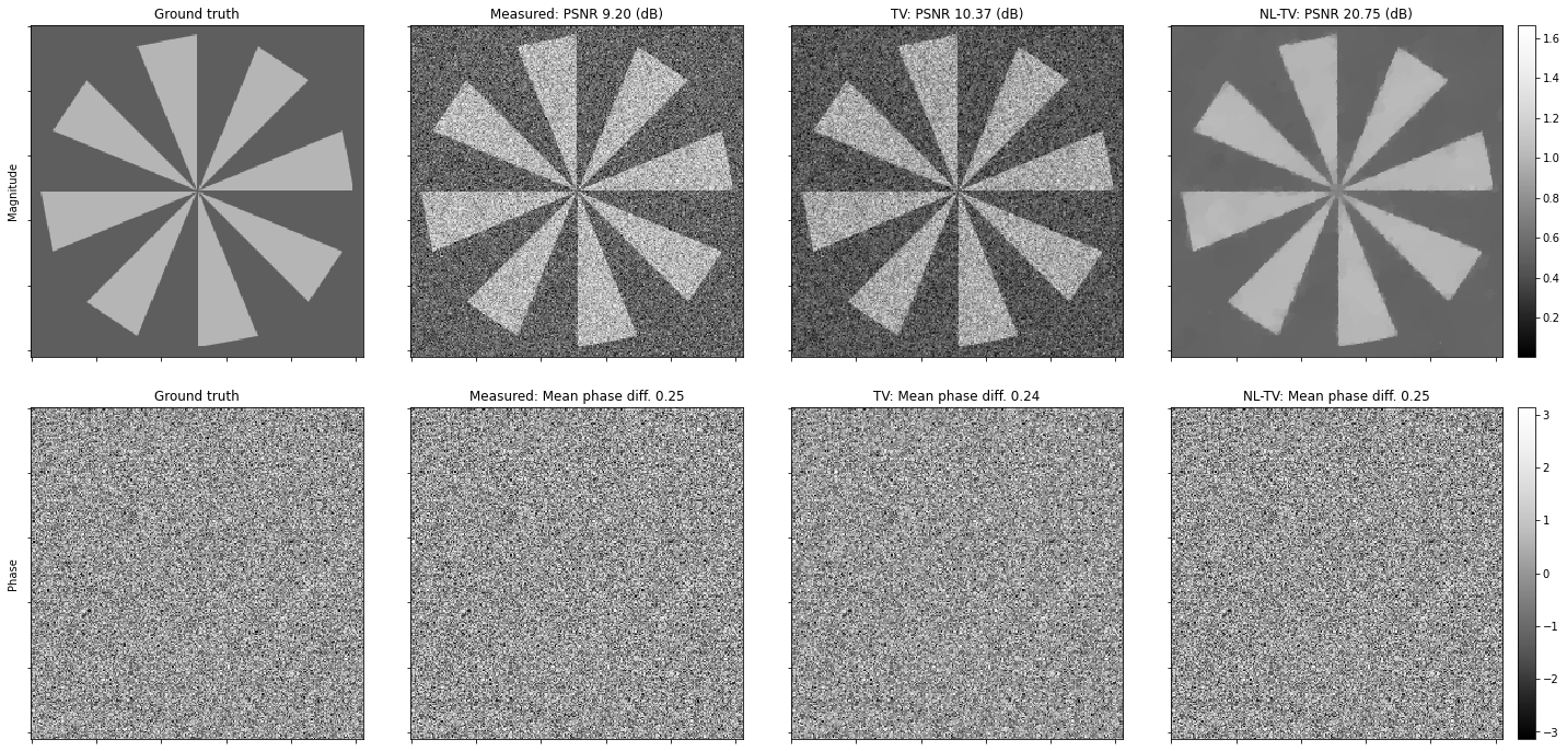
where \(\mathbf{y}\) is the measurement, \(\|\cdot\|_{2,1}\) is the \(\ell_{2,1}\) mixed norm, and \(C\) is a non-linear operator that applies a linear difference operator to the magnitude of a complex array. The standard TV solution, which is also computed for comparison purposes, gives very poor results since the difference is applied independently to real and imaginary components of the complex image.
[1]:
from mpl_toolkits.axes_grid1 import make_axes_locatable
from xdesign import SiemensStar, discrete_phantom

import scico.numpy as snp
import scico.random
from scico import functional, linop, loss, metric, operator, plot
from scico.examples import phase_diff
from scico.optimize import PDHG
from scico.util import device_info
plot.config_notebook_plotting()
Create a ground truth image.
[2]:
N = 256  # image size
phantom = SiemensStar(16)
x_mag = snp.pad(discrete_phantom(phantom, N - 16), 8) + 1.0
x_mag /= x_mag.max()
# Create reference image with structured magnitude and random phase
x_gt = x_mag * snp.exp(-1j * scico.random.randn(x_mag.shape, seed=0)[0])
Add noise to create a noisy test image.
[3]:
σ = 0.25  # noise standard deviation
noise, key = scico.random.randn(x_gt.shape, seed=1, dtype=snp.complex64)
y = x_gt + σ * noise
Denoise with standard total variation.
[4]:
λ_tv = 6e-2
f = loss.SquaredL2Loss(y=y)
g = λ_tv * functional.L21Norm()
# The append=0 option makes the results of horizontal and vertical finite
# differences the same shape, which is required for the L21Norm.
C = linop.FiniteDifference(input_shape=x_gt.shape, input_dtype=snp.complex64, append=0)
solver_tv = PDHG(
    f=f,
    g=g,
    C=C,
    tau=4e-1,
    sigma=4e-1,
    maxiter=200,
    itstat_options={"display": True, "period": 10},
)
print(f"Solving on {device_info()}\n")
x_tv = solver_tv.solve()
hist_tv = solver_tv.itstat_object.history(transpose=True)
Solving on GPU (NVIDIA GeForce RTX 2080 Ti)

Iter  Time      Objective  Prml Rsdl  Dual Rsdl
-----------------------------------------------
   0  2.29e+00  1.066e+04  1.373e+02  3.829e+01
  10  3.42e+00  3.814e+03  4.043e+00  1.280e-02
  20  3.47e+00  3.806e+03  1.398e-01  6.217e-04
  30  3.52e+00  3.806e+03  4.831e-03  4.037e-05
  40  3.57e+00  3.806e+03  1.670e-04  2.078e-05
  50  3.63e+00  3.806e+03  7.106e-06  1.361e-05
  60  3.68e+00  3.806e+03  1.948e-06  1.236e-05
  70  3.73e+00  3.806e+03  1.580e-06  1.228e-05
  80  3.78e+00  3.806e+03  1.532e-06  1.227e-05
  90  3.82e+00  3.806e+03  1.563e-06  1.222e-05
 100  3.86e+00  3.806e+03  1.511e-06  1.231e-05
 110  3.90e+00  3.806e+03  1.545e-06  1.223e-05
 120  3.93e+00  3.806e+03  1.547e-06  1.225e-05
 130  3.97e+00  3.806e+03  1.539e-06  1.227e-05
 140  4.00e+00  3.806e+03  1.524e-06  1.227e-05
 150  4.04e+00  3.806e+03  1.537e-06  1.221e-05
 160  4.07e+00  3.806e+03  1.511e-06  1.230e-05
 170  4.11e+00  3.806e+03  1.540e-06  1.225e-05
 180  4.14e+00  3.806e+03  1.533e-06  1.226e-05
 190  4.18e+00  3.806e+03  1.542e-06  1.227e-05
 199  4.22e+00  3.806e+03  1.527e-06  1.223e-05
Denoise with total variation applied to the magnitude of a complex image.
[5]:
λ_nltv = 2e-1
g = λ_nltv * functional.L21Norm()
# Redefine C for real input (now applied to magnitude of a complex array)
C = linop.FiniteDifference(input_shape=x_gt.shape, input_dtype=snp.float32, append=0)
# Operator computing differences of absolute values
D = C @ operator.Abs(input_shape=x_gt.shape, input_dtype=snp.complex64)
solver_nltv = PDHG(
    f=f,
    g=g,
    C=D,
    tau=4e-1,
    sigma=4e-1,
    maxiter=200,
    itstat_options={"display": True, "period": 10},
)
x_nltv = solver_nltv.solve()
hist_nltv = solver_nltv.itstat_object.history(transpose=True)
Iter  Time      Objective  Prml Rsdl  Dual Rsdl
-----------------------------------------------
   0  1.38e+00  1.056e+04  1.373e+02  5.088e+01
  10  1.94e+00  1.214e+03  4.852e+00  2.524e+00
  20  2.02e+00  1.164e+03  4.825e-01  1.097e+00
  30  2.10e+00  1.154e+03  2.040e-01  7.021e-01
  40  2.17e+00  1.150e+03  1.215e-01  5.130e-01
  50  2.22e+00  1.148e+03  8.232e-02  4.049e-01
  60  2.28e+00  1.146e+03  6.026e-02  3.324e-01
  70  2.33e+00  1.145e+03  4.652e-02  2.803e-01
  80  2.38e+00  1.145e+03  3.700e-02  2.420e-01
  90  2.43e+00  1.144e+03  3.054e-02  2.120e-01
 100  2.48e+00  1.144e+03  2.535e-02  1.885e-01
 110  2.54e+00  1.143e+03  2.157e-02  1.695e-01
 120  2.59e+00  1.143e+03  1.869e-02  1.536e-01
 130  2.65e+00  1.143e+03  1.618e-02  1.401e-01
 140  2.70e+00  1.143e+03  1.422e-02  1.286e-01
 150  2.75e+00  1.142e+03  1.237e-02  1.190e-01
 160  2.80e+00  1.142e+03  1.121e-02  1.105e-01
 170  2.85e+00  1.142e+03  9.792e-03  1.035e-01
 180  2.91e+00  1.142e+03  8.941e-03  9.702e-02
 190  2.96e+00  1.142e+03  8.485e-03  9.119e-02
 199  3.01e+00  1.142e+03  7.614e-03  8.665e-02
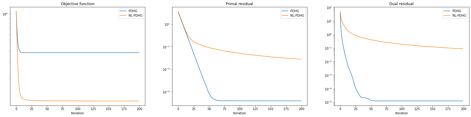
Plot results.
[6]:
fig, ax = plot.subplots(nrows=1, ncols=3, sharex=True, sharey=False, figsize=(27, 6))
plot.plot(
    snp.vstack((hist_tv.Objective, hist_nltv.Objective)).T,
    ptyp="semilogy",
    title="Objective function",
    xlbl="Iteration",
    lgnd=("PDHG", "NL-PDHG"),
    fig=fig,
    ax=ax[0],
)
plot.plot(
    snp.vstack((hist_tv.Prml_Rsdl, hist_nltv.Prml_Rsdl)).T,
    ptyp="semilogy",
    title="Primal residual",
    xlbl="Iteration",
    lgnd=("PDHG", "NL-PDHG"),
    fig=fig,
    ax=ax[1],
)
plot.plot(
    snp.vstack((hist_tv.Dual_Rsdl, hist_nltv.Dual_Rsdl)).T,
    ptyp="semilogy",
    title="Dual residual",
    xlbl="Iteration",
    lgnd=("PDHG", "NL-PDHG"),
    fig=fig,
    ax=ax[2],
)
fig.show()


fig, ax = plot.subplots(nrows=2, ncols=4, figsize=(20, 10))
norm = plot.matplotlib.colors.Normalize(
    vmin=min(snp.abs(x_gt).min(), snp.abs(y).min(), snp.abs(x_tv).min(), snp.abs(x_nltv).min()),
    vmax=max(snp.abs(x_gt).max(), snp.abs(y).max(), snp.abs(x_tv).max(), snp.abs(x_nltv).max()),
)
plot.imview(snp.abs(x_gt), title="Ground truth", cbar=None, fig=fig, ax=ax[0, 0], norm=norm)
plot.imview(
    snp.abs(y),
    title="Measured: PSNR %.2f (dB)" % metric.psnr(snp.abs(x_gt), snp.abs(y)),
    cbar=None,
    fig=fig,
    ax=ax[0, 1],
    norm=norm,
)
plot.imview(
    snp.abs(x_tv),
    title="TV: PSNR %.2f (dB)" % metric.psnr(snp.abs(x_gt), snp.abs(x_tv)),
    cbar=None,
    fig=fig,
    ax=ax[0, 2],
    norm=norm,
)
plot.imview(
    snp.abs(x_nltv),
    title="NL-TV: PSNR %.2f (dB)" % metric.psnr(snp.abs(x_gt), snp.abs(x_nltv)),
    cbar=None,
    fig=fig,
    ax=ax[0, 3],
    norm=norm,
)
divider = make_axes_locatable(ax[0, 3])
cax = divider.append_axes("right", size="5%", pad=0.2)
fig.colorbar(ax[0, 3].get_images()[0], cax=cax)
norm = plot.matplotlib.colors.Normalize(
    vmin=min(snp.angle(x_gt).min(), snp.angle(x_tv).min(), snp.angle(x_nltv).min()),
    vmax=max(snp.angle(x_gt).max(), snp.angle(x_tv).max(), snp.angle(x_nltv).max()),
)
plot.imview(
    snp.angle(x_gt),
    title="Ground truth",
    cbar=None,
    fig=fig,
    ax=ax[1, 0],
    norm=norm,
)
plot.imview(
    snp.angle(y),
    title="Measured: Mean phase diff. %.2f" % phase_diff(snp.angle(x_gt), snp.angle(y)).mean(),
    cbar=None,
    fig=fig,
    ax=ax[1, 1],
    norm=norm,
)
plot.imview(
    snp.angle(x_tv),
    title="TV: Mean phase diff. %.2f" % phase_diff(snp.angle(x_gt), snp.angle(x_tv)).mean(),
    cbar=None,
    fig=fig,
    ax=ax[1, 2],
    norm=norm,
)
plot.imview(
    snp.angle(x_nltv),
    title="NL-TV: Mean phase diff. %.2f" % phase_diff(snp.angle(x_gt), snp.angle(x_nltv)).mean(),
    cbar=None,
    fig=fig,
    ax=ax[1, 3],
    norm=norm,
)
divider = make_axes_locatable(ax[1, 3])
cax = divider.append_axes("right", size="5%", pad=0.2)
fig.colorbar(ax[1, 3].get_images()[0], cax=cax)
ax[0, 0].set_ylabel("Magnitude")
ax[1, 0].set_ylabel("Phase")
fig.tight_layout()
fig.show()