Parameter Tuning for Image Deconvolution with TV Regularization (ADMM Solver)

This example demonstrates the use of scico.ray.tune to tune parameters for the companion example script. The ray.tune function API is used in this example.

This script is hard-coded to run on CPU only to avoid the large number of warnings that are emitted when GPU resources are requested but not available, and due to the difficulty of supressing these warnings in a way that does not force use of the CPU only. To enable GPU usage, comment out the os.environ statements near the beginning of the script, and change the value of the “gpu” entry in the resources dict from 0 to 1. Note that two environment variables are set to suppress the warnings because JAX_PLATFORMS was intended to replace JAX_PLATFORM_NAME but this change has yet to be correctly implemented (see google/jax#6805 and google/jax#10272).

# isort: off
import os

os.environ["JAX_PLATFORM_NAME"] = "cpu"
os.environ["JAX_PLATFORMS"] = "cpu"


from xdesign import SiemensStar, discrete_phantom

import scico.numpy as snp
import scico.random
from scico import functional, linop, loss, metric, plot
from scico.optimize.admm import ADMM, LinearSubproblemSolver
from scico.ray import report, tune
plot.config_notebook_plotting()

Create a ground truth image.

phantom = SiemensStar(32)
N = 256  # image size
x_gt = snp.pad(discrete_phantom(phantom, N - 16), 8)

Set up the forward operator and create a test signal consisting of a blurred signal with additive Gaussian noise.

n = 5  # convolution kernel size
σ = 20.0 / 255  # noise level

psf = snp.ones((n, n)) / (n * n)
A = linop.Convolve(h=psf, input_shape=x_gt.shape)

Ax = A(x_gt)  # blurred image
noise, key = scico.random.randn(Ax.shape, seed=0)
y = Ax + σ * noise

Define performance evaluation function.

def eval_params(config, x_gt, psf, y):
    """Parameter evaluation function. The `config` parameter is a
    dict of specific parameters for evaluation of a single parameter
    set (a pair of parameters in this case). The remaining parameters
    are objects that are passed to the evaluation function via the
    ray object store.
    """
    # Extract solver parameters from config dict.
    λ, ρ = config["lambda"], config["rho"]
    # Set up problem to be solved.
    A = linop.Convolve(h=psf, input_shape=x_gt.shape)
    f = loss.SquaredL2Loss(y=y, A=A)
    g = λ * functional.L21Norm()
    C = linop.FiniteDifference(input_shape=x_gt.shape, append=0)
    # Define solver.
    solver = ADMM(
        f=f,
        g_list=[g],
        C_list=[C],
        rho_list=[ρ],
        x0=A.adj(y),
        maxiter=10,
        subproblem_solver=LinearSubproblemSolver(),
    )
    # Perform 50 iterations, reporting performance to ray.tune every 10 iterations.
    for step in range(5):
        x_admm = solver.solve()
        report({"psnr": float(metric.psnr(x_gt, x_admm))})

Define parameter search space and resources per trial.

config = {"lambda": tune.loguniform(1e-3, 1e-1), "rho": tune.loguniform(1e-2, 1e0)}
resources = {"cpu": 4, "gpu": 0}  # cpus per trial, gpus per trial

Run parameter search.

tuner = tune.Tuner(
    tune.with_parameters(eval_params, x_gt=x_gt, psf=psf, y=y),
    param_space=config,
    resources=resources,
    metric="psnr",
    mode="max",
    num_samples=100,  # perform 100 parameter evaluations
)
results = tuner.fit()

P:   0 R:   0 T: 100  psnr: 2.23e+01 at lambda: 2.10e-02, rho: 1.39e-01

Display best parameters and corresponding performance.

best_result = results.get_best_result()
best_config = best_result.config
print(f"Best PSNR: {best_result.metrics['psnr']:.2f} dB")
print("Best config: " + ", ".join([f"{k}: {v:.2e}" for k, v in best_config.items()]))

Best PSNR: 22.30 dB
Best config: lambda: 2.10e-02, rho: 1.39e-01

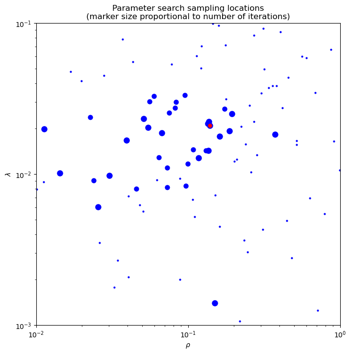
Plot parameter values visited during parameter search. Marker sizes are proportional to number of iterations run at each parameter pair. The best point in the parameter space is indicated in red.

fig = plot.figure(figsize=(8, 8))
trials = results.get_dataframe()
for t in trials.iloc:
    n = t["training_iteration"]
    plot.plot(
        t["config/lambda"],
        t["config/rho"],
        ptyp="loglog",
        lw=0,
        ms=(0.5 + 1.5 * n),
        marker="o",
        mfc="blue",
        mec="blue",
        fig=fig,
    )
plot.plot(
    best_config["lambda"],
    best_config["rho"],
    ptyp="loglog",
    title="Parameter search sampling locations\n(marker size proportional to number of iterations)",
    xlbl=r"$\rho$",
    ylbl=r"$\lambda$",
    lw=0,
    ms=5.0,
    marker="o",
    mfc="red",
    mec="red",
    fig=fig,
)
ax = fig.axes[0]
ax.set_xlim([config["rho"].lower, config["rho"].upper])
ax.set_ylim([config["lambda"].lower, config["lambda"].upper])
fig.show()

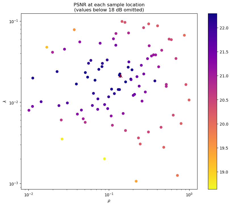
Plot parameter values visited during parameter search and corresponding reconstruction PSNRs.The best point in the parameter space is indicated in red.

𝜌 = [t["config/rho"] for t in trials.iloc]
𝜆 = [t["config/lambda"] for t in trials.iloc]
psnr = [t["psnr"] for t in trials.iloc]
minpsnr = min(max(psnr), 18.0)
𝜌, 𝜆, psnr = zip(*filter(lambda x: x[2] >= minpsnr, zip(𝜌, 𝜆, psnr)))
fig, ax = plot.subplots(figsize=(10, 8))
sc = ax.scatter(𝜌, 𝜆, c=psnr, cmap=plot.cm.plasma_r)
fig.colorbar(sc)
plot.plot(
    best_config["lambda"],
    best_config["rho"],
    ptyp="loglog",
    lw=0,
    ms=12.0,
    marker="2",
    mfc="red",
    mec="red",
    fig=fig,
    ax=ax,
)
ax.set_xscale("log")
ax.set_yscale("log")
ax.set_xlabel(r"$\rho$")
ax.set_ylabel(r"$\lambda$")
ax.set_title("PSNR at each sample location\n(values below 18 dB omitted)")
fig.show()