Total Variation Denoising (ADMM)

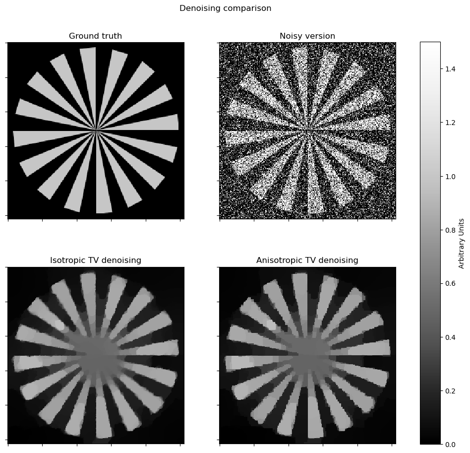
This example compares denoising via isotropic and anisotropic total variation (TV) regularization [50] [27]. It solves the denoising problem

\[\mathrm{argmin}_{\mathbf{x}} \; (1/2) \| \mathbf{y} - \mathbf{x} \|_2^2 + \lambda R(\mathbf{x}) \;,\]

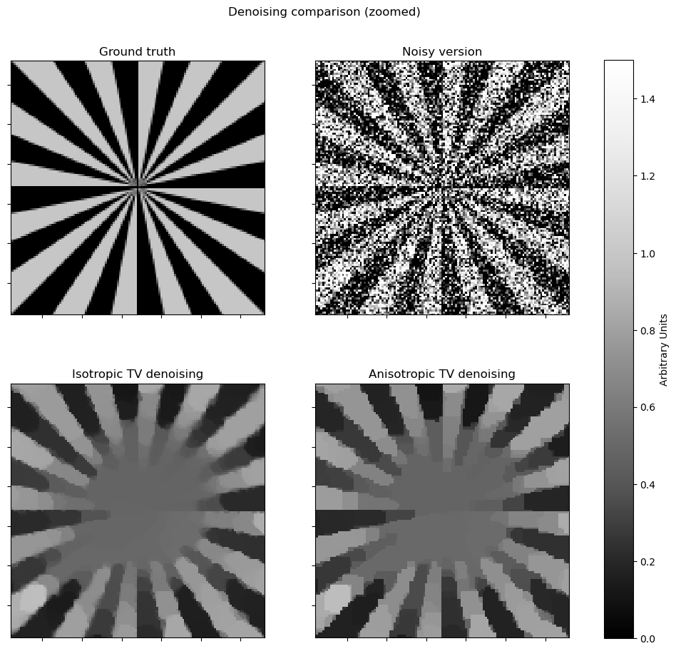
where \(R\) is either the isotropic or anisotropic TV regularizer. In SCICO, switching between these two regularizers involves a one-line change: replacing an L1Norm with a L21Norm. Note that the isotropic version exhibits fewer block-like artifacts on edges that are not vertical or horizontal.

import komplot as kplt
from xdesign import SiemensStar, discrete_phantom

import scico.numpy as snp
import scico.random
from scico import functional, linop, loss
from scico.optimize.admm import ADMM, LinearSubproblemSolver
from scico.util import device_info
kplt.config_notebook_plotting()

Create a ground truth image.

N = 256  # image size
phantom = SiemensStar(16)
x_gt = snp.pad(discrete_phantom(phantom, N - 16), 8)
x_gt = x_gt / x_gt.max()

Add noise to create a noisy test image.

σ = 0.75  # noise standard deviation
noise, key = scico.random.randn(x_gt.shape, seed=0)
y = x_gt + σ * noise

Denoise with isotropic total variation.

λ_iso = 1.4e0
f = loss.SquaredL2Loss(y=y)
g_iso = λ_iso * functional.L21Norm()

# The append=0 option makes the results of horizontal and vertical finite
# differences the same shape, which is required for the L21Norm.
C = linop.FiniteDifference(input_shape=x_gt.shape, append=0)
solver = ADMM(
    f=f,
    g_list=[g_iso],
    C_list=[C],
    rho_list=[1e1],
    x0=y,
    maxiter=100,
    subproblem_solver=LinearSubproblemSolver(cg_kwargs={"tol": 1e-3, "maxiter": 20}),
    itstat_options={"display": True, "period": 10},
)

print(f"Solving on {device_info()}\n")
solver.solve()
x_iso = solver.x
print()

Solving on GPU (NVIDIA GeForce RTX 2080 Ti)

Iter  Time      Objective  Prml Rsdl  Dual Rsdl  CG It  CG Res
-----------------------------------------------------------------
   0  2.32e+00  1.082e+05  1.130e+02  7.370e+02      0  0.000e+00
  10  3.63e+00  3.879e+04  1.613e+01  4.378e+02     12  9.056e-04
  20  4.13e+00  2.319e+04  9.525e+00  1.367e+02     15  8.979e-04
  30  4.56e+00  2.218e+04  2.745e+00  2.872e+01     11  9.789e-04
  40  4.90e+00  2.215e+04  1.123e+00  7.784e+00      8  8.381e-04
  50  5.17e+00  2.216e+04  7.083e-01  2.510e+00      3  9.077e-04
  60  5.36e+00  2.217e+04  4.900e-01  1.508e+00      2  7.916e-04
  70  5.51e+00  2.217e+04  3.638e-01  9.179e-01      2  9.830e-04
  80  5.67e+00  2.217e+04  2.862e-01  5.203e-01      1  9.438e-04
  90  5.79e+00  2.217e+04  2.314e-01  5.204e-01      2  7.694e-04
  99  5.89e+00  2.217e+04  2.011e-01  3.766e-01      1  8.711e-04

Denoise with anisotropic total variation for comparison.

# Tune the weight to give the same data fidelity as the isotropic case.
λ_aniso = 1.2e0
g_aniso = λ_aniso * functional.L1Norm()

solver = ADMM(
    f=f,
    g_list=[g_aniso],
    C_list=[C],
    rho_list=[1e1],
    x0=y,
    maxiter=100,
    subproblem_solver=LinearSubproblemSolver(cg_kwargs={"tol": 1e-3, "maxiter": 20}),
    itstat_options={"display": True, "period": 10},
)

solver.solve()
x_aniso = solver.x
print()

Iter  Time      Objective  Prml Rsdl  Dual Rsdl  CG It  CG Res
-----------------------------------------------------------------
   0  1.08e-01  1.161e+05  1.330e+02  8.474e+02      0  0.000e+00
  10  7.27e-01  3.675e+04  2.230e+01  4.373e+02     13  9.376e-04
  20  1.31e+00  2.289e+04  9.372e+00  1.186e+02     15  8.551e-04
  30  1.74e+00  2.217e+04  2.686e+00  2.639e+01     10  9.899e-04
  40  2.00e+00  2.214e+04  1.111e+00  8.613e+00      7  9.888e-04
  50  2.20e+00  2.214e+04  6.627e-01  3.744e+00      3  9.860e-04
  60  2.38e+00  2.215e+04  4.299e-01  2.360e+00      4  9.621e-04
  70  2.54e+00  2.215e+04  3.020e-01  1.585e+00      2  7.335e-04
  80  2.66e+00  2.215e+04  2.281e-01  1.169e+00      2  6.168e-04
  90  2.80e+00  2.215e+04  1.870e-01  7.254e-01      1  8.881e-04
  99  2.92e+00  2.215e+04  1.584e-01  4.521e-01      1  9.551e-04

Compute and print the data fidelity.

for x, name in zip((x_iso, x_aniso), ("Isotropic", "Anisotropic")):
    df = f(x)
    print(f"Data fidelity for {name} TV was {df:.2e}")

Data fidelity for Isotropic TV was 1.92e+04
Data fidelity for Anisotropic TV was 1.91e+04

Plot results.

plt_args = dict(norm=kplt.colors.Normalize(vmin=0, vmax=1.5))
fig, ax = kplt.subplots(nrows=2, ncols=2, sharex=True, sharey=True, figsize=(11, 10))
kplt.imview(x_gt, title="Ground truth", ax=ax[0, 0], **plt_args)
kplt.imview(y, title="Noisy version", ax=ax[0, 1], **plt_args)
kplt.imview(x_iso, title="Isotropic TV denoising", ax=ax[1, 0], **plt_args)
kplt.imview(x_aniso, title="Anisotropic TV denoising", ax=ax[1, 1], **plt_args)
fig.subplots_adjust(left=0.1, right=0.99, top=0.95, bottom=0.05, wspace=0.2, hspace=0.01)
fig.colorbar(
    ax[0, 0].get_images()[0], ax=ax, location="right", shrink=0.9, pad=0.05, label="Arbitrary Units"
)
fig.suptitle("Denoising comparison")
fig.show()

# zoomed version
fig, ax = kplt.subplots(nrows=2, ncols=2, sharex=True, sharey=True, figsize=(11, 10))
kplt.imview(x_gt, title="Ground truth", ax=ax[0, 0], **plt_args)
kplt.imview(y, title="Noisy version", ax=ax[0, 1], **plt_args)
kplt.imview(x_iso, title="Isotropic TV denoising", ax=ax[1, 0], **plt_args)
kplt.imview(x_aniso, title="Anisotropic TV denoising", ax=ax[1, 1], **plt_args)
ax[0, 0].set_xlim(N // 4, N // 4 + N // 2)
ax[0, 0].set_ylim(N // 4, N // 4 + N // 2)
fig.subplots_adjust(left=0.1, right=0.99, top=0.95, bottom=0.05, wspace=0.2, hspace=0.01)
fig.colorbar(
    ax[0, 0].get_images()[0], ax=ax, location="right", shrink=0.9, pad=0.05, label="Arbitrary Units"
)
fig.suptitle("Denoising comparison (zoomed)")
fig.show()