TV-Regularized Sparse-View CT Reconstruction (Integrated Projector)

This example demonstrates solution of a sparse-view CT reconstruction problem with isotropic total variation (TV) regularization

\[\mathrm{argmin}_{\mathbf{x}} \; (1/2) \| \mathbf{y} - A \mathbf{x} \|_2^2 + \lambda \| C \mathbf{x} \|_{2,1} \;,\]

where \(A\) is the X-ray transform (the CT forward projection operator), \(\mathbf{y}\) is the sinogram, \(C\) is a 2D finite difference operator, and \(\mathbf{x}\) is the reconstructed image. This example uses the CT projector integrated into scico, while the companion example script uses the projector provided by the astra package.

import numpy as np

from mpl_toolkits.axes_grid1 import make_axes_locatable
from xdesign import Foam, discrete_phantom

import scico.numpy as snp
from scico import functional, linop, loss, metric, plot
from scico.linop.xray import XRayTransform2D
from scico.optimize.admm import ADMM, LinearSubproblemSolver
from scico.util import device_info
plot.config_notebook_plotting()

Create a ground truth image.

N = 512  # phantom size
np.random.seed(1234)
x_gt = snp.array(discrete_phantom(Foam(size_range=[0.075, 0.0025], gap=1e-3, porosity=1), size=N))

Configure CT projection operator and generate synthetic measurements.

n_projection = 45  # number of projections
angles = np.linspace(0, np.pi, n_projection, endpoint=False)  # evenly spaced projection angles
det_count = int(N * 1.05 / np.sqrt(2.0))
dx = 1.0 / np.sqrt(2)
A = XRayTransform2D(
    (N, N), angles + np.pi / 2.0, det_count=det_count, dx=dx
)  # CT projection operator
y = A @ x_gt  # sinogram

Set up problem functional and ADMM solver object.

λ = 2e0  # ℓ1 norm regularization parameter
ρ = 5e0  # ADMM penalty parameter
maxiter = 25  # number of ADMM iterations
cg_tol = 1e-4  # CG relative tolerance
cg_maxiter = 25  # maximum CG iterations per ADMM iteration

# The append=0 option makes the results of horizontal and vertical
# finite differences the same shape, which is required for the L21Norm,
# which is used so that g(Cx) corresponds to isotropic TV.
C = linop.FiniteDifference(input_shape=x_gt.shape, append=0)
g = λ * functional.L21Norm()
f = loss.SquaredL2Loss(y=y, A=A)
x0 = snp.clip(A.fbp(y), 0, 1.0)

solver = ADMM(
    f=f,
    g_list=[g],
    C_list=[C],
    rho_list=[ρ],
    x0=x0,
    maxiter=maxiter,
    subproblem_solver=LinearSubproblemSolver(cg_kwargs={"tol": cg_tol, "maxiter": cg_maxiter}),
    itstat_options={"display": True, "period": 5},
)

Run the solver.

print(f"Solving on {device_info()}\n")
solver.solve()
hist = solver.itstat_object.history(transpose=True)
x_reconstruction = snp.clip(solver.x, 0, 1.0)

Solving on GPU (NVIDIA GeForce RTX 2080 Ti)

Iter  Time      Objective  Prml Rsdl  Dual Rsdl  CG It  CG Res
-----------------------------------------------------------------
   0  1.50e+00  1.645e+03  1.800e+02  8.801e+02     20  8.979e-05
   5  2.42e+00  2.152e+04  4.778e+01  6.793e+01     15  8.194e-05
  10  2.62e+00  2.671e+04  4.353e+01  5.245e+01     16  9.137e-05
  15  2.79e+00  2.736e+04  1.908e+01  3.565e+01     15  6.610e-05
  20  2.89e+00  2.761e+04  5.344e+01  4.783e+01     13  8.792e-05
  24  2.97e+00  2.801e+04  1.513e+01  7.396e+00      1  9.906e-05

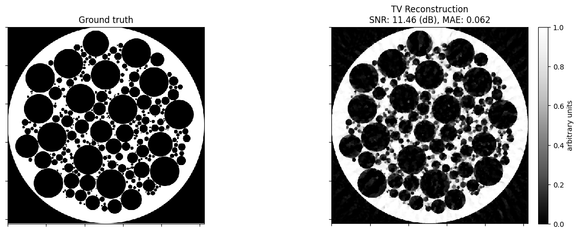
Show the recovered image.

fig, ax = plot.subplots(nrows=1, ncols=3, figsize=(15, 5))
plot.imview(x_gt, title="Ground truth", cbar=None, fig=fig, ax=ax[0])
plot.imview(
    x0,
    title="FBP Reconstruction: \nSNR: %.2f (dB), MAE: %.3f"
    % (metric.snr(x_gt, x0), metric.mae(x_gt, x0)),
    cbar=None,
    fig=fig,
    ax=ax[1],
)
plot.imview(
    x_reconstruction,
    title="TV Reconstruction\nSNR: %.2f (dB), MAE: %.3f"
    % (metric.snr(x_gt, x_reconstruction), metric.mae(x_gt, x_reconstruction)),
    fig=fig,
    ax=ax[2],
)
divider = make_axes_locatable(ax[2])
cax = divider.append_axes("right", size="5%", pad=0.2)
fig.colorbar(ax[2].get_images()[0], cax=cax, label="arbitrary units")
fig.show()

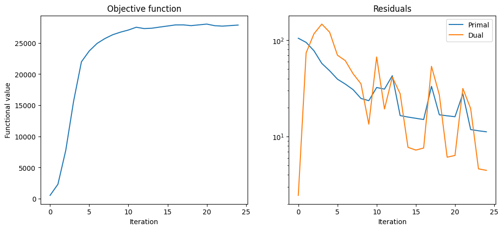
Plot convergence statistics.

fig, ax = plot.subplots(nrows=1, ncols=2, figsize=(12, 5))
plot.plot(
    hist.Objective,
    title="Objective function",
    xlbl="Iteration",
    ylbl="Functional value",
    fig=fig,
    ax=ax[0],
)
plot.plot(
    snp.vstack((hist.Prml_Rsdl, hist.Dual_Rsdl)).T,
    ptyp="semilogy",
    title="Residuals",
    xlbl="Iteration",
    lgnd=("Primal", "Dual"),
    fig=fig,
    ax=ax[1],
)
fig.show()