Image Deconvolution with TV Regularization (Proximal ADMM Solver)

This example demonstrates the solution of an image deconvolution problem with isotropic total variation (TV) regularization

\[\mathrm{argmin}_{\mathbf{x}} \; (1/2) \| \mathbf{y} - C \mathbf{x} \|_2^2 + \lambda \| D \mathbf{x} \|_{2,1} \;,\]

where \(C\) is a convolution operator, \(\mathbf{y}\) is the blurred image, \(D\) is a 2D finite difference operator, and \(\mathbf{x}\) is the deconvolved image.

In this example the problem is solved via proximal ADMM, while standard ADMM is used in a companion example.

import komplot as kplt
from xdesign import SiemensStar, discrete_phantom

import scico.numpy as snp
import scico.random
from scico import functional, linop, loss, metric
from scico.optimize import ProximalADMM
from scico.util import device_info
kplt.config_notebook_plotting()

Create a ground truth image.

phantom = SiemensStar(32)
N = 256  # image size
x_gt = snp.pad(discrete_phantom(phantom, N - 16), 8)

Set up the forward operator and create a test signal consisting of a blurred signal with additive Gaussian noise.

n = 5  # convolution kernel size
σ = 20.0 / 255  # noise level

psf = snp.ones((n, n)) / (n * n)
C = linop.Convolve(h=psf, input_shape=x_gt.shape)

Cx = C(x_gt)  # blurred image
noise, key = scico.random.randn(Cx.shape, seed=0)
y = Cx + σ * noise

Set up the problem to be solved. We want to minimize the functional

\[\mathrm{argmin}_{\mathbf{x}} \; (1/2) \| \mathbf{y} - C \mathbf{x} \|_2^2 + \lambda \| D \mathbf{x} \|_{2,1} \;,\]

where \(C\) is the convolution operator and \(D\) is a finite difference operator. This problem can be expressed as

\[\mathrm{argmin}_{\mathbf{x}, \mathbf{z}} \; (1/2) \| \mathbf{y} - \mathbf{z}_0 \|_2^2 + \lambda \| \mathbf{z}_1 \|_{2,1} \;\; \text{such that} \;\; \mathbf{z}_0 = C \mathbf{x} \;\; \text{and} \;\; \mathbf{z}_1 = D \mathbf{x} \;,\]

which can be written in the form of a standard ADMM problem

\[\mathrm{argmin}_{\mathbf{x}, \mathbf{z}} \; f(\mathbf{x}) + g(\mathbf{z}) \;\; \text{such that} \;\; A \mathbf{x} + B \mathbf{z} = \mathbf{c}\]

with

\[f = 0 \qquad g = g_0 + g_1\]

\[g_0(\mathbf{z}_0) = (1/2) \| \mathbf{y} - \mathbf{z}_0 \|_2^2 \qquad g_1(\mathbf{z}_1) = \lambda \| \mathbf{z}_1 \|_{2,1}\]

\[\begin{split}A = \left( \begin{array}{c} C \\ D \end{array} \right) \qquad B = \left( \begin{array}{cc} -I & 0 \\ 0 & -I \end{array} \right) \qquad \mathbf{c} = \left( \begin{array}{c} 0 \\ 0 \end{array} \right) \;.\end{split}\]

This is a more complex splitting than that used in the companion example, but it allows the use of a proximal ADMM solver in a way that avoids the need for the conjugate gradient sub-iterations used by the ADMM solver in the companion example.

f = functional.ZeroFunctional()
g0 = loss.SquaredL2Loss(y=y)
λ = 2.0e-2  # ℓ2,1 norm regularization parameter
g1 = λ * functional.L21Norm()
g = functional.SeparableFunctional((g0, g1))

D = linop.FiniteDifference(input_shape=x_gt.shape, append=0)
A = linop.VerticalStack((C, D))

Set up a proximal ADMM solver object.

ρ = 5.0e-2  # ADMM penalty parameter
maxiter = 50  # number of ADMM iterations
mu, nu = ProximalADMM.estimate_parameters(A)

solver = ProximalADMM(
    f=f,
    g=g,
    A=A,
    B=None,
    rho=ρ,
    mu=mu,
    nu=nu,
    x0=C.adj(y),
    maxiter=maxiter,
    itstat_options={"display": True, "period": 10},
)

Run the solver.

print(f"Solving on {device_info()}\n")
x = solver.solve()
hist = solver.itstat_object.history(transpose=True)

Solving on GPU (NVIDIA GeForce RTX 2080 Ti)

Iter  Time      Objective  Prml Rsdl  Dual Rsdl
-----------------------------------------------
   0  1.25e+00  1.161e+00  3.894e+01  1.308e+02
  10  2.52e+00  1.783e+02  1.552e+01  3.489e+00
  20  2.70e+00  2.145e+02  8.852e+00  2.538e+00
  30  2.88e+00  2.496e+02  5.304e+00  1.220e+00
  40  3.11e+00  2.787e+02  3.315e+00  7.807e-01
  49  3.32e+00  2.936e+02  2.150e+00  5.076e-01

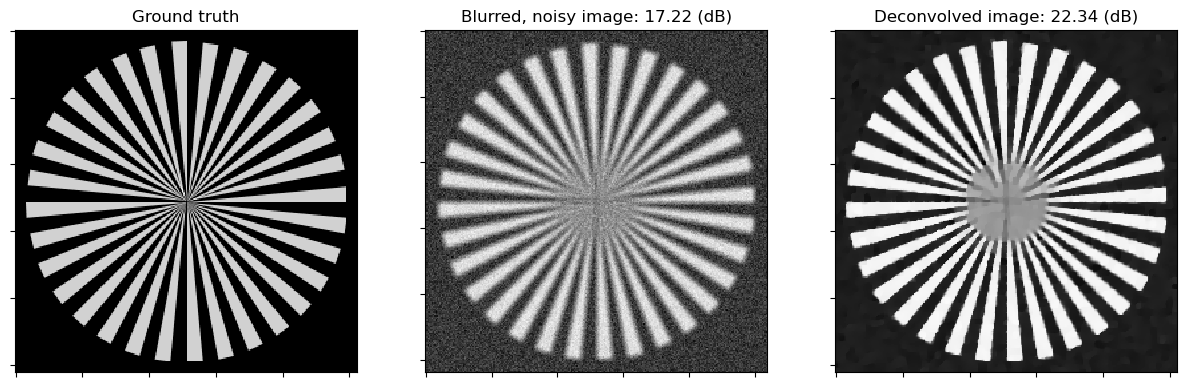
Show the recovered image.

fig, ax = kplt.subplots(nrows=1, ncols=3, sharex=True, sharey=True, figsize=(15, 5))
kplt.imview(x_gt, cmap="Blues", title="Ground truth", ax=ax[0])
nc = n // 2
yc = y[nc:-nc, nc:-nc]
kplt.imview(
    y, cmap="Blues", title="Blurred, noisy image: %.2f (dB)" % metric.psnr(x_gt, yc), ax=ax[1]
)
kplt.imview(
    solver.x,
    cmap="Blues",
    title="Deconvolved image: %.2f (dB)" % metric.psnr(x_gt, solver.x),
    ax=ax[2],
)
fig.show()

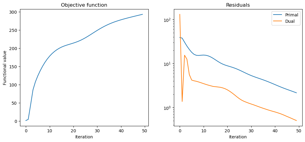
Plot convergence statistics.

fig, ax = kplt.subplots(nrows=1, ncols=2, figsize=(12, 5))
kplt.plot(
    hist.Objective,
    title="Objective function",
    xlabel="Iteration",
    ylabel="Functional value",
    ax=ax[0],
)
kplt.plot(
    snp.array((hist.Prml_Rsdl, hist.Dual_Rsdl)).T,
    ylog=True,
    title="Residuals",
    xlabel="Iteration",
    legend=("Primal", "Dual"),
    ax=ax[1],
)
fig.show()