PPP (with BM3D) Image Deconvolution (ADMM Solver)

This example demonstrates the solution of an image deconvolution problem using the ADMM Plug-and-Play Priors (PPP) algorithm [56], with the BM3D [17] denoiser.

import numpy as np

import komplot as kplt
from xdesign import Foam, discrete_phantom

import scico.numpy as snp
from scico import functional, linop, loss, metric, random
from scico.optimize.admm import ADMM, LinearSubproblemSolver
from scico.util import device_info
kplt.config_notebook_plotting()

Create a ground truth image.

np.random.seed(1234)
N = 512  # image size
x_gt = discrete_phantom(Foam(size_range=[0.075, 0.0025], gap=1e-3, porosity=1), size=N)
x_gt = snp.array(x_gt)  # convert to jax array

Set up forward operator and test signal consisting of blurred signal with additive Gaussian noise.

n = 5  # convolution kernel size
σ = 20.0 / 255  # noise level

psf = snp.ones((n, n)) / (n * n)
A = linop.Convolve(h=psf, input_shape=x_gt.shape)

Ax = A(x_gt)  # blurred image
noise, key = random.randn(Ax.shape)
y = Ax + σ * noise

Set up ADMM solver.

f = loss.SquaredL2Loss(y=y, A=A)
C = linop.Identity(x_gt.shape)

λ = 20.0 / 255  # BM3D regularization strength
g = λ * functional.BM3D()

ρ = 1.0  # ADMM penalty parameter
maxiter = 10  # number of ADMM iterations

solver = ADMM(
    f=f,
    g_list=[g],
    C_list=[C],
    rho_list=[ρ],
    x0=A.T @ y,
    maxiter=maxiter,
    subproblem_solver=LinearSubproblemSolver(cg_kwargs={"tol": 1e-3, "maxiter": 100}),
    itstat_options={"display": True},
)

Run the solver.

print(f"Solving on {device_info()}\n")
x = solver.solve()
x = snp.clip(x, 0, 1)
hist = solver.itstat_object.history(transpose=True)

Solving on GPU (NVIDIA GeForce RTX 2080 Ti)

Iter  Time      Prml Rsdl  Dual Rsdl  CG It  CG Res
------------------------------------------------------
   0  4.31e+00  9.566e+00  1.463e+01      3  2.077e-04
   1  7.06e+00  3.677e+00  9.177e+00      3  2.275e-04
   2  1.07e+01  1.225e+00  6.477e+00      2  6.779e-04
   3  1.48e+01  8.981e-01  4.750e+00      2  4.347e-04
   4  2.02e+01  7.582e-01  3.669e+00      2  3.154e-04
   5  2.46e+01  6.767e-01  2.965e+00      2  2.339e-04
   6  2.88e+01  6.322e-01  2.480e+00      2  1.786e-04
   7  3.56e+01  5.247e-01  2.064e+00      1  8.090e-04
   8  4.28e+01  5.394e-01  1.825e+00      1  5.616e-04
   9  4.98e+01  5.240e-01  1.632e+00      1  5.274e-04

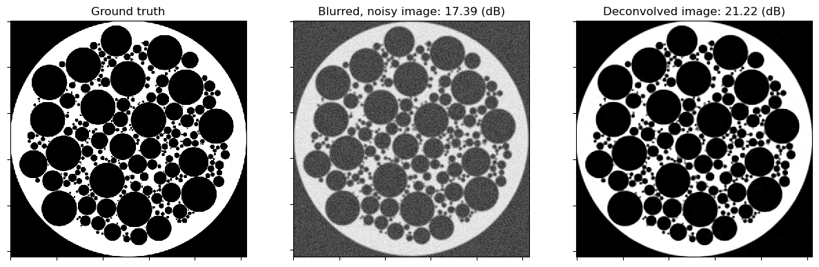
Show the recovered image.

fig, ax = kplt.subplots(nrows=1, ncols=3, sharex=True, sharey=True, figsize=(15, 5))
kplt.imview(x_gt, cmap="Blues", title="Ground truth", ax=ax[0])
nc = n // 2
yc = snp.clip(y[nc:-nc, nc:-nc], 0, 1)
kplt.imview(
    y, cmap="Blues", title="Blurred, noisy image: %.2f (dB)" % metric.psnr(x_gt, yc), ax=ax[1]
)
kplt.imview(x, cmap="Blues", title="Deconvolved image: %.2f (dB)" % metric.psnr(x_gt, x), ax=ax[2])
fig.show()

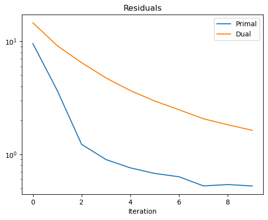
Plot convergence statistics.

kplt.plot(
    snp.array((hist.Prml_Rsdl, hist.Dual_Rsdl)).T,
    ylog=True,
    title="Residuals",
    xlabel="Iteration",
    legend=("Primal", "Dual"),
)

<komplot.LinePlot at 0x78b96c6e79e0>