TV-Regularized Abel Inversion

This example demonstrates a total variation (TV) regularized Abel inversion by solving the problem

\[\mathrm{argmin}_{\mathbf{x}} \; (1/2) \| \mathbf{y} - A \mathbf{x} \|_2^2 + \lambda \| C \mathbf{x} \|_1 \;,\]

where \(A\) is the Abel projector (with an implementation based on a projector from PyAbel [25]), \(\mathbf{y}\) is the measured data, \(C\) is a 2D finite difference operator, and \(\mathbf{x}\) is the solution.

import numpy as np

import komplot as kplt

import scico.numpy as snp
from scico import functional, linop, loss, metric
from scico.examples import create_circular_phantom
from scico.linop.xray.abel import AbelTransform
from scico.optimize.admm import ADMM, LinearSubproblemSolver
from scico.util import device_info
kplt.config_notebook_plotting()

Create a ground truth image.

N = 256  # image size
x_gt = create_circular_phantom((N, N), [0.4 * N, 0.2 * N, 0.1 * N], [1, 0, 0.5])

Set up the forward operator and create a test measurement.

A = AbelTransform(x_gt.shape)
y = A @ x_gt
np.random.seed(12345)
y = y + np.random.normal(size=y.shape).astype(np.float32)

Compute inverse Abel transform solution.

x_inv = A.inverse(y)

Set up the problem to be solved. Anisotropic TV, which gives slightly better performance than isotropic TV for this problem, is used here.

f = loss.SquaredL2Loss(y=y, A=A)
λ = 2.35e1  # ℓ1 norm regularization parameter
g = λ * functional.L1Norm()  # Note the use of anisotropic TV
C = linop.FiniteDifference(input_shape=x_gt.shape)

Set up ADMM solver object.

ρ = 1.03e2  # ADMM penalty parameter
maxiter = 100  # number of ADMM iterations
cg_tol = 1e-4  # CG relative tolerance
cg_maxiter = 25  # maximum CG iterations per ADMM iteration

solver = ADMM(
    f=f,
    g_list=[g],
    C_list=[C],
    rho_list=[ρ],
    x0=snp.clip(x_inv, 0.0, 1.0),
    maxiter=maxiter,
    subproblem_solver=LinearSubproblemSolver(cg_kwargs={"tol": cg_tol, "maxiter": cg_maxiter}),
    itstat_options={"display": True, "period": 10},
)

Run the solver.

print(f"Solving on {device_info()}\n")
solver.solve()
x_tv = snp.clip(solver.x, 0.0, 1.0)

Solving on GPU (NVIDIA GeForce RTX 2080 Ti)

Iter  Time      Objective  Prml Rsdl  Dual Rsdl  CG It  CG Res
-----------------------------------------------------------------
   0  2.31e+00  5.897e+04  3.531e+02  7.648e+03     17  9.734e-05
  10  3.77e+00  5.973e+04  1.650e+01  6.834e+01      5  7.628e-05
  20  3.94e+00  6.132e+04  8.719e+00  6.872e+00      0  8.422e-05
  30  4.11e+00  6.182e+04  1.139e+01  3.056e+01      4  4.874e-05
  40  4.27e+00  6.209e+04  5.933e+00  1.786e+01      4  7.998e-05
  50  4.40e+00  6.224e+04  3.701e+00  2.907e+00      0  9.522e-05
  60  4.56e+00  6.247e+04  8.009e+00  2.692e+01      3  4.132e-05
  70  4.72e+00  6.259e+04  5.332e+00  4.006e+00      0  8.825e-05
  80  4.86e+00  6.262e+04  3.140e+00  2.437e+00      0  9.594e-05
  90  4.96e+00  6.269e+04  5.823e+00  3.170e+00      0  9.493e-05
  99  5.06e+00  6.271e+04  2.199e+00  1.344e+00      0  7.553e-05

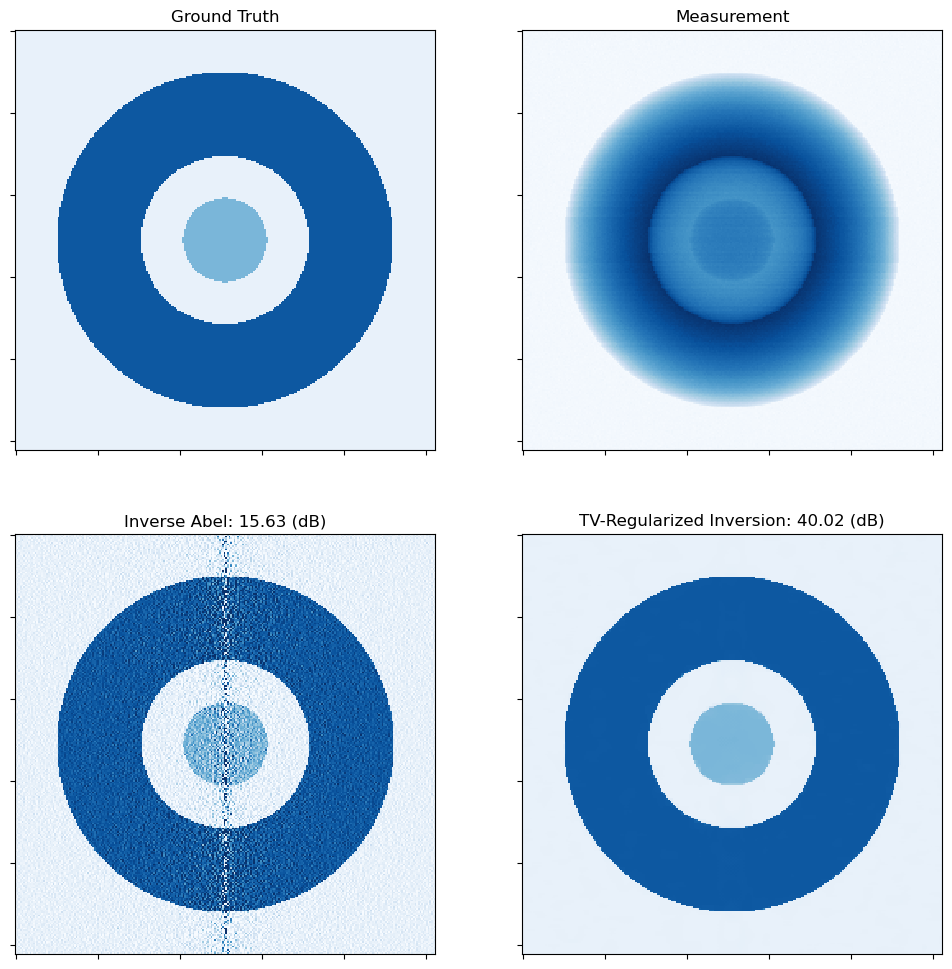
Show results.

norm = kplt.colors.Normalize(vmin=-0.1, vmax=1.2)
fig, ax = kplt.subplots(nrows=2, ncols=2, figsize=(12, 12))
kplt.imview(x_gt, title="Ground Truth", cmap=kplt.cm.Blues, ax=ax[0, 0], norm=norm)
kplt.imview(y, title="Measurement", cmap=kplt.cm.Blues, ax=ax[0, 1])
kplt.imview(
    x_inv,
    title="Inverse Abel: %.2f (dB)" % metric.psnr(x_gt, x_inv),
    cmap=kplt.cm.Blues,
    ax=ax[1, 0],
    norm=norm,
)
kplt.imview(
    x_tv,
    title="TV-Regularized Inversion: %.2f (dB)" % metric.psnr(x_gt, x_tv),
    cmap=kplt.cm.Blues,
    ax=ax[1, 1],
    norm=norm,
)
fig.show()