TV-Regularized Sparse-View CT Reconstruction (Multiple Projectors)
This example demonstrates solution of a sparse-view CT reconstruction problem with isotropic total variation (TV) regularization
where \(A\) is the X-ray transform (the CT forward projection operator), \(\mathbf{y}\) is the sinogram, \(C\) is a 2D finite difference operator, and \(\mathbf{x}\) is the reconstructed image. The solution is computed and compared for all three 2D CT projectors available in scico, using a sinogram computed with the astra projector.
[1]:
import numpy as np

import komplot as kplt
from xdesign import Foam, discrete_phantom

import scico.numpy as snp
from scico import functional, linop, loss, metric
from scico.linop.xray import XRayTransform2D, astra, svmbir
from scico.optimize.admm import ADMM, LinearSubproblemSolver
from scico.util import device_info
kplt.config_notebook_plotting()
Create a ground truth image.
[2]:
N = 512  # phantom size
np.random.seed(1234)
x_gt = snp.array(discrete_phantom(Foam(size_range=[0.075, 0.0025], gap=1e-3, porosity=1), size=N))
Define CT geometry and construct array of (approximately) equivalent projectors.
[3]:
n_projection = 45  # number of projections
angles = np.linspace(0, np.pi, n_projection, endpoint=False)  # evenly spaced projection angles
det_count = int(N * 1.05 / np.sqrt(2.0))
det_spacing = np.sqrt(2)
projectors = {
    "astra": astra.XRayTransform2D(
        x_gt.shape, det_count, det_spacing, angles - np.pi / 2.0
    ),  # astra
    "svmbir": svmbir.XRayTransform(
        x_gt.shape, 2 * np.pi - angles, det_count, delta_pixel=1.0, delta_channel=det_spacing
    ),  # svmbir
    "scico": XRayTransform2D((N, N), angles, det_count=det_count, dx=1 / det_spacing),  # scico
}
Compute common sinogram using astra projector.
[4]:
A = projectors["astra"]
noise = np.random.normal(size=(n_projection, det_count)).astype(np.float32)
y = A @ x_gt + 2.0 * noise
Construct initial solution for regularized problem.
[5]:
x0 = A.fbp(y)
Solve the same problem using the different projectors.
[6]:
print(f"Solving on {device_info()}")
x_rec, hist = {}, {}
for p in projectors.keys():
    print(f"\nSolving with {p} projector")

    # Set up ADMM solver object.
    λ = 2e1  # L1 norm regularization parameter
    ρ = 1e3  # ADMM penalty parameter
    maxiter = 100  # number of ADMM iterations
    cg_tol = 1e-4  # CG relative tolerance
    cg_maxiter = 50  # maximum CG iterations per ADMM iteration

    # The append=0 option makes the results of horizontal and vertical
    # finite differences the same shape, which is required for the L21Norm,
    # which is used so that g(Cx) corresponds to isotropic TV.
    C = linop.FiniteDifference(input_shape=x_gt.shape, append=0)
    g = λ * functional.L21Norm()
    A = projectors[p]
    f = loss.SquaredL2Loss(y=y, A=A)

    # Set up the solver.
    solver = ADMM(
        f=f,
        g_list=[g],
        C_list=[C],
        rho_list=[ρ],
        x0=x0,
        maxiter=maxiter,
        subproblem_solver=LinearSubproblemSolver(cg_kwargs={"tol": cg_tol, "maxiter": cg_maxiter}),
        itstat_options={"display": True, "period": 5},
    )

    # Run the solver.
    solver.solve()
    hist[p] = solver.itstat_object.history(transpose=True)
    x_rec[p] = solver.x

    if p == "scico":
        x_rec[p] = x_rec[p] * det_spacing  # to match ASTRA's scaling
Solving on GPU (NVIDIA GeForce RTX 2080 Ti)

Solving with astra projector
Iter  Time      Objective  Prml Rsdl  Dual Rsdl  CG It  CG Res
-----------------------------------------------------------------
   0  3.86e+00  2.882e+06  3.234e+02  3.891e+04     28  7.134e-05
   5  8.37e+00  7.071e+05  5.774e+01  1.926e+04     12  9.686e-05
  10  1.17e+01  3.556e+05  5.925e+01  1.001e+04     14  9.365e-05
  15  1.55e+01  2.880e+05  3.673e+01  4.758e+03     13  9.191e-05
  20  1.91e+01  2.721e+05  2.110e+01  2.504e+03     11  8.894e-05
  25  2.23e+01  2.666e+05  1.322e+01  1.553e+03      7  9.867e-05
  30  2.48e+01  2.640e+05  8.747e+00  1.126e+03      6  9.464e-05
  35  2.69e+01  2.625e+05  6.351e+00  9.087e+02      5  9.423e-05
  40  2.87e+01  2.616e+05  5.191e+00  7.200e+02      4  9.547e-05
  45  3.04e+01  2.610e+05  3.830e+00  6.485e+02      4  9.715e-05
  50  3.22e+01  2.605e+05  2.935e+00  5.761e+02      3  9.936e-05
  55  3.38e+01  2.601e+05  2.344e+00  5.210e+02      3  8.713e-05
  60  3.55e+01  2.598e+05  2.205e+00  4.682e+02      3  8.724e-05
  65  3.70e+01  2.596e+05  2.478e+00  4.053e+02      2  9.821e-05
  70  3.83e+01  2.594e+05  2.649e+00  3.238e+02      1  9.411e-05
  75  4.00e+01  2.592e+05  2.067e+00  3.516e+02      2  9.189e-05
  80  4.14e+01  2.591e+05  2.776e+00  2.785e+02      2  9.461e-05
  85  4.29e+01  2.590e+05  2.685e+00  2.586e+02      2  8.997e-05
  90  4.43e+01  2.589e+05  2.587e+00  2.458e+02      2  8.916e-05
  95  4.58e+01  2.588e+05  2.268e+00  2.437e+02      2  8.612e-05
  99  4.68e+01  2.588e+05  2.186e+00  2.370e+02      2  8.413e-05

Solving with svmbir projector
Iter  Time      Objective  Prml Rsdl  Dual Rsdl  CG It  CG Res
-----------------------------------------------------------------
   0  1.66e+02  2.428e+06  3.234e+02  3.682e+04     23  9.924e-05
   5  5.93e+02  7.055e+05  5.333e+01  1.864e+04     11  9.773e-05
  10  8.97e+02  3.847e+05  5.653e+01  1.024e+04     13  9.074e-05
  15  1.14e+03  3.058e+05  3.704e+01  5.165e+03     12  9.418e-05
  20  1.31e+03  2.837e+05  2.264e+01  2.808e+03     10  9.474e-05
  25  1.46e+03  2.756e+05  1.423e+01  1.751e+03      8  9.431e-05
  30  1.58e+03  2.718e+05  9.402e+00  1.264e+03      7  9.231e-05
  35  1.69e+03  2.697e+05  7.119e+00  9.896e+02      5  9.805e-05
  40  1.77e+03  2.685e+05  5.458e+00  8.117e+02      5  9.245e-05
  45  1.84e+03  2.676e+05  4.121e+00  6.940e+02      3  9.939e-05
  50  1.91e+03  2.669e+05  3.255e+00  6.182e+02      3  9.799e-05
  55  1.98e+03  2.665e+05  3.226e+00  5.479e+02      4  8.408e-05
  60  2.04e+03  2.661e+05  2.202e+00  5.118e+02      3  8.841e-05
  65  2.11e+03  2.657e+05  2.095e+00  4.645e+02      3  8.296e-05
  70  2.16e+03  2.655e+05  1.873e+00  4.352e+02      2  9.970e-05
  75  2.22e+03  2.653e+05  2.557e+00  3.651e+02      2  9.436e-05
  80  2.27e+03  2.651e+05  2.851e+00  3.051e+02      2  9.455e-05
  85  2.33e+03  2.650e+05  2.729e+00  2.895e+02      2  9.595e-05
  90  2.38e+03  2.649e+05  2.634e+00  2.704e+02      2  8.870e-05
  95  2.43e+03  2.648e+05  2.547e+00  2.583e+02      2  8.931e-05
  99  2.47e+03  2.647e+05  2.293e+00  1.797e+02      1  9.134e-05

Solving with scico projector
Iter  Time      Objective  Prml Rsdl  Dual Rsdl  CG It  CG Res
-----------------------------------------------------------------
   0  1.34e+00  2.902e+06  3.233e+02  5.525e+04     24  9.663e-05
   5  1.71e+00  5.083e+05  6.554e+01  1.878e+04     11  8.385e-05
  10  2.07e+00  2.649e+05  5.835e+01  8.844e+03     13  8.634e-05
  15  2.43e+00  2.186e+05  3.320e+01  4.079e+03     12  8.207e-05
  20  2.70e+00  2.068e+05  1.878e+01  2.186e+03      8  9.506e-05
  25  2.93e+00  2.025e+05  1.215e+01  1.387e+03      5  9.851e-05
  30  3.13e+00  2.005e+05  7.831e+00  1.053e+03      6  8.939e-05
  35  3.28e+00  1.994e+05  5.337e+00  8.306e+02      4  9.508e-05
  40  3.44e+00  1.986e+05  3.956e+00  7.134e+02      4  9.890e-05
  45  3.58e+00  1.981e+05  3.418e+00  6.182e+02      3  9.677e-05
  50  3.73e+00  1.977e+05  3.074e+00  5.563e+02      3  9.502e-05
  55  3.87e+00  1.973e+05  3.253e+00  4.776e+02      3  8.172e-05
  60  4.01e+00  1.971e+05  2.912e+00  3.611e+02      2  9.694e-05
  65  4.14e+00  1.969e+05  3.179e+00  3.071e+02      2  7.341e-05
  70  4.25e+00  1.968e+05  2.989e+00  2.249e+02      1  9.421e-05
  75  4.36e+00  1.967e+05  2.740e+00  2.504e+02      2  7.334e-05
  80  4.47e+00  1.966e+05  2.417e+00  1.796e+02      1  9.748e-05
  85  4.58e+00  1.965e+05  2.209e+00  2.312e+02      2  7.319e-05
  90  4.69e+00  1.965e+05  2.022e+00  1.547e+02      1  9.115e-05
  95  4.80e+00  1.964e+05  1.805e+00  2.116e+02      2  7.261e-05
  99  4.89e+00  1.964e+05  1.652e+00  2.067e+02      2  7.229e-05
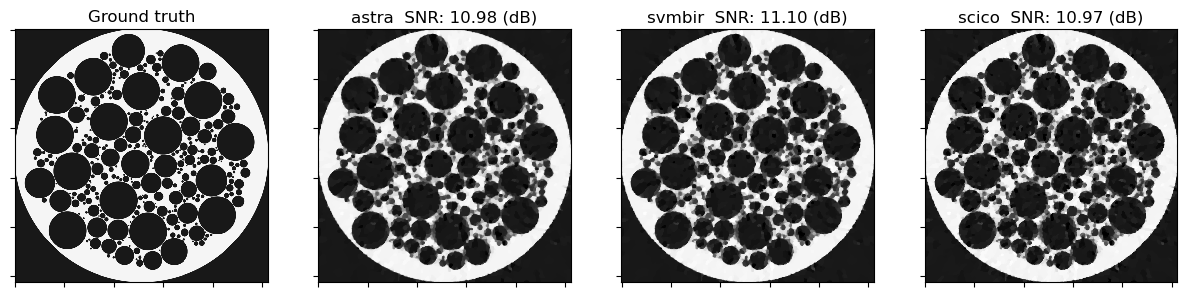
Compare reconstruction results.
[7]:
print("Reconstruction SNR:")
for p in projectors.keys():
    print(f"  {(p + ':'):7s}  {metric.snr(x_gt, x_rec[p]):5.2f} dB")
Reconstruction SNR:
  astra:   10.98 dB
  svmbir:  11.10 dB
  scico:   10.96 dB
Display sinogram.
[8]:
fig, ax = kplt.subplots(nrows=1, ncols=1, figsize=(15, 3))
kplt.imview(y, cmap="Blues", title="sinogram", ax=ax)
fig.show()

Plot convergence statistics.
[9]:
fig, ax = kplt.subplots(nrows=1, ncols=3, figsize=(12, 5))
kplt.plot(
    np.array([hist[p].Objective for p in projectors.keys()]).T,
    title="Objective function",
    xlabel="Iteration",
    ylabel="Functional value",
    legend=projectors.keys(),
    ax=ax[0],
)
kplt.plot(
    np.array([hist[p].Prml_Rsdl for p in projectors.keys()]).T,
    ylog=True,
    title="Primal Residual",
    xlabel="Iteration",
    ax=ax[1],
)
kplt.plot(
    np.array([hist[p].Dual_Rsdl for p in projectors.keys()]).T,
    ylog=True,
    title="Dual Residual",
    xlabel="Iteration",
    ax=ax[2],
)
fig.show()

Show the recovered images.
[10]:
fig, ax = kplt.subplots(nrows=1, ncols=4, sharex=True, sharey=True, figsize=(15, 5))
kplt.imview(x_gt, cmap="Blues", title="Ground truth", ax=ax[0])
for n, p in enumerate(projectors.keys()):
    kplt.imview(
        x_rec[p],
        cmap="Blues",
        title="%s  SNR: %.2f (dB)" % (p, metric.snr(x_gt, x_rec[p])),
        ax=ax[n + 1],
    )
for ax in ax:
    ax.get_images()[0].set_clim(-0.1, 1.1)
fig.tight_layout()
fig.show()