Circulant Blur Image Deconvolution with TV Regularization

This example demonstrates the solution of an image deconvolution problem with isotropic total variation (TV) regularization

\[\mathrm{argmin}_{\mathbf{x}} \; (1/2) \| \mathbf{y} - A \mathbf{x} \|_2^2 + \lambda \| C \mathbf{x} \|_{2,1} \;,\]

where \(A\) is a circular convolution operator, \(\mathbf{y}\) is the blurred image, \(C\) is a 2D finite difference operator, and \(\mathbf{x}\) is the deconvolved image.

import komplot as kplt
from xdesign import SiemensStar, discrete_phantom

import scico.numpy as snp
import scico.random
from scico import functional, linop, loss, metric
from scico.optimize.admm import ADMM, CircularConvolveSolver
from scico.util import device_info
kplt.config_notebook_plotting()

Create a ground truth image.

phantom = SiemensStar(32)
N = 256  # image size
x_gt = snp.pad(discrete_phantom(phantom, N - 16), 8)

Set up the forward operator and create a test signal consisting of a blurred signal with additive Gaussian noise.

n = 5  # convolution kernel size
σ = 20.0 / 255  # noise level

psf = snp.ones((n, n)) / (n * n)
A = linop.CircularConvolve(h=psf, input_shape=x_gt.shape)

Ax = A(x_gt)  # blurred image
noise, key = scico.random.randn(Ax.shape, seed=0)
y = Ax + σ * noise

Set up an ADMM solver object.

λ = 2e-2  # ℓ2,1 norm regularization parameter
ρ = 5e-1  # ADMM penalty parameter
maxiter = 50  # number of ADMM iterations

f = loss.SquaredL2Loss(y=y, A=A)
# Penalty parameters must be accounted for in the gi functions, not as
# additional inputs.
g = λ * functional.L21Norm()  # regularization functionals gi
C = linop.FiniteDifference(x_gt.shape, circular=True)
solver = ADMM(
    f=f,
    g_list=[g],
    C_list=[C],
    rho_list=[ρ],
    x0=A.adj(y),
    maxiter=maxiter,
    subproblem_solver=CircularConvolveSolver(),
    itstat_options={"display": True, "period": 10},
)

Run the solver.

print(f"Solving on {device_info()}\n")
x = solver.solve()
hist = solver.itstat_object.history(transpose=True)

Solving on GPU (NVIDIA GeForce RTX 2080 Ti)

Iter  Time      Objective  Prml Rsdl  Dual Rsdl
-----------------------------------------------
   0  1.12e+00  3.256e+02  6.303e+00  4.047e+00
  10  2.35e+00  3.268e+02  2.952e-01  1.024e+00
  20  2.43e+00  3.235e+02  1.308e-01  6.186e-01
  30  2.49e+00  3.222e+02  7.545e-02  4.323e-01
  40  2.54e+00  3.215e+02  4.939e-02  3.202e-01
  49  2.59e+00  3.212e+02  3.729e-02  2.541e-01

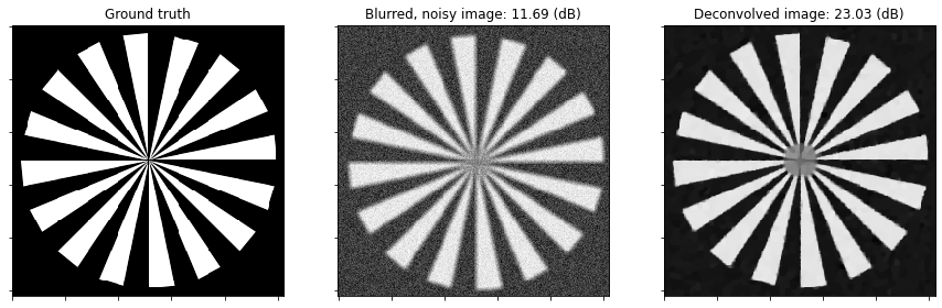
Show the recovered image.

fig, ax = kplt.subplots(nrows=1, ncols=3, sharex=True, sharey=True, figsize=(15, 5))
kplt.imview(x_gt, cmap="Blues", title="Ground truth", ax=ax[0])
kplt.imview(
    y, cmap="Blues", title="Blurred, noisy image: %.2f (dB)" % metric.psnr(x_gt, y), ax=ax[1]
)
kplt.imview(x, cmap="Blues", title="Deconvolved image: %.2f (dB)" % metric.psnr(x_gt, x), ax=ax[2])
fig.show()

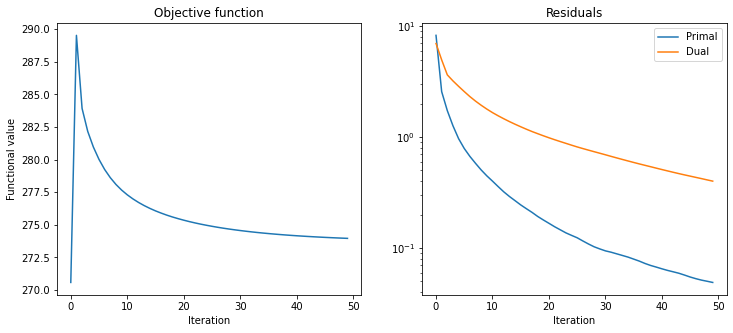
Plot convergence statistics.

fig, ax = kplt.subplots(nrows=1, ncols=2, figsize=(12, 5))
kplt.plot(
    hist.Objective,
    title="Objective function",
    xlabel="Iteration",
    ylabel="Functional value",
    ax=ax[0],
)
kplt.plot(
    snp.array((hist.Prml_Rsdl, hist.Dual_Rsdl)).T,
    ylog=True,
    title="Residuals",
    xlabel="Iteration",
    legend=("Primal", "Dual"),
    ax=ax[1],
)
fig.show()