TV-Regularized Cone Beam CT for Symmetric Objects
This example demonstrates a total variation (TV) regularized reconstruction for cone beam CT of a cylindrically symmetric object, by solving the problem
where \(C\) is a single-view X-ray transform (with an implementation based on a projector from the AXITOM package [45]), \(\mathbf{y}\) is the measured data, \(D\) is a 2D finite difference operator, and \(\mathbf{x}\) is the solution.
[1]:
import numpy as np

import komplot as kplt

import scico.numpy as snp
from scico import functional, linop, loss, metric
from scico.examples import create_circular_phantom
from scico.linop.xray.symcone import SymConeXRayTransform
from scico.optimize import ProximalADMM
from scico.util import device_info
kplt.config_notebook_plotting()
Create a ground truth image.
[2]:
N = 256  # image size
x_gt = create_circular_phantom((N, N), [0.4 * N, 0.2 * N, 0.1 * N], [1, 0, 0.5])
Set up the forward operator and create a test measurement.
[3]:
C = SymConeXRayTransform(x_gt.shape, obj_dist=5e2 * N, det_dist=6e2 * N, num_slabs=4)
y = C @ x_gt
np.random.seed(12345)
y = y + np.random.normal(size=y.shape).astype(np.float32)
Compute FDK reconstruction.
[4]:
x_inv = C.fdk(y)
Set up problem and solver. We want to minimize the functional
where \(C\) is the X-ray transform and \(D\) is a finite difference operator. We use anisotropic TV, which gives slightly better performance than isotropic TV in this case. This problem can be expressed as
which can be written in the form of a standard ADMM problem
with
[5]:
𝛼 = 7e1  # improve problem conditioning by balancing C and D components of A
λ = 8e0  # ℓ1 norm regularization parameter
ρ = 1e-2  # ADMM penalty parameter
maxiter = 250  # number of ADMM iterations

f = functional.ZeroFunctional()
g0 = loss.SquaredL2Loss(y=y)
g1 = (λ / 𝛼) * functional.L1Norm()
g = functional.SeparableFunctional((g0, g1))
D = linop.FiniteDifference(input_shape=x_gt.shape, append=0)

A = linop.VerticalStack((C, 𝛼 * D))
mu, nu = ProximalADMM.estimate_parameters(A, maxiter=20)

solver = ProximalADMM(
    f=f,
    g=g,
    A=A,
    B=None,
    rho=ρ,
    mu=mu,
    nu=nu,
    x0=snp.clip(x_inv, 0.0, 1.0),
    maxiter=maxiter,
    itstat_options={"display": True, "period": 20},
)
Run the solver.
[6]:
print(f"Solving on {device_info()}\n")
x_tv = solver.solve()
hist = solver.itstat_object.history(transpose=True)
Solving on GPU (NVIDIA GeForce RTX 2080 Ti)

Iter  Time      Objective  Prml Rsdl  Dual Rsdl
-----------------------------------------------
   0  1.06e+00  9.618e+03  1.520e+03  1.913e+04
  20  2.18e+00  1.244e+04  2.479e+02  4.733e+01
  40  2.51e+00  1.471e+04  1.870e+02  3.463e+01
  60  2.86e+00  1.738e+04  1.567e+02  2.181e+01
  80  3.20e+00  2.078e+04  1.243e+02  1.486e+01
 100  3.58e+00  2.375e+04  1.022e+02  1.000e+01
 120  4.02e+00  2.669e+04  8.874e+01  6.690e+00
 140  4.43e+00  2.922e+04  6.702e+01  6.931e+00
 160  4.80e+00  3.156e+04  5.728e+01  5.942e+00
 180  5.13e+00  3.338e+04  4.897e+01  4.662e+00
 200  5.48e+00  3.497e+04  3.626e+01  4.353e+00
 220  5.83e+00  3.624e+04  3.389e+01  3.582e+00
 240  6.21e+00  3.736e+04  2.810e+01  3.051e+00
 249  6.39e+00  3.783e+04  2.379e+01  2.901e+00
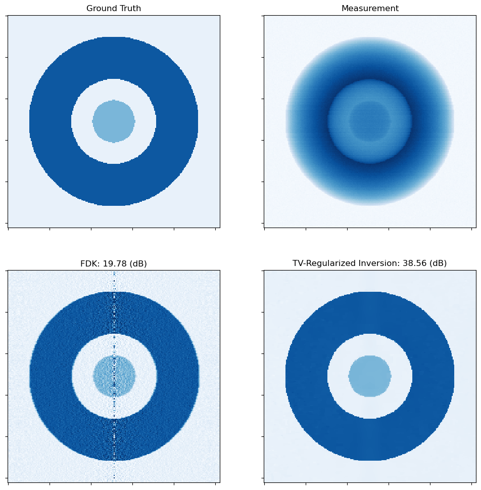
Show results.
[7]:
norm = kplt.colors.Normalize(vmin=-0.1, vmax=1.2)
fig, ax = kplt.subplots(nrows=2, ncols=2, sharex=True, sharey=True, figsize=(12, 12))
kplt.imview(x_gt, title="Ground Truth", cmap=kplt.cm.Blues, ax=ax[0, 0], norm=norm)
kplt.imview(y, title="Measurement", cmap=kplt.cm.Blues, ax=ax[0, 1])
kplt.imview(
    x_inv,
    title="FDK: %.2f (dB)" % metric.psnr(x_gt, x_inv),
    cmap=kplt.cm.Blues,
    ax=ax[1, 0],
    norm=norm,
)
kplt.imview(
    x_tv,
    title="TV-Regularized Inversion: %.2f (dB)" % metric.psnr(x_gt, x_tv),
    cmap=kplt.cm.Blues,
    ax=ax[1, 1],
    norm=norm,
)
fig.show()
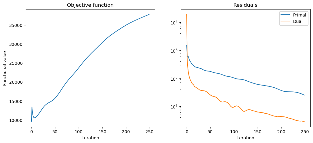
Plot convergence statistics.
[8]:
fig, ax = kplt.subplots(nrows=1, ncols=2, figsize=(12, 5))
kplt.plot(
    hist.Objective,
    title="Objective function",
    xlabel="Iteration",
    ylabel="Functional value",
    ax=ax[0],
)
kplt.plot(
    snp.array((hist.Prml_Rsdl, hist.Dual_Rsdl)).T,
    ylog=True,
    title="Residuals",
    xlabel="Iteration",
    legend=("Primal", "Dual"),
    ax=ax[1],
)
fig.show()