3D TV-Regularized Sparse-View CT Reconstruction (ADMM Solver)
This example demonstrates solution of a sparse-view, 3D CT reconstruction problem with isotropic total variation (TV) regularization
\[\mathrm{argmin}_{\mathbf{x}} \; (1/2) \| \mathbf{y} - C \mathbf{x}
\|_2^2 + \lambda \| D \mathbf{x} \|_{2,1} \;,\]
where \(C\) is the X-ray transform (the CT forward projection operator), \(\mathbf{y}\) is the sinogram, \(D\) is a 3D finite difference operator, and \(\mathbf{x}\) is the reconstructed image.
In this example the problem is solved via ADMM, while proximal ADMM is used in a companion example.
[1]:
import numpy as np

import komplot as kplt
from mpl_toolkits.axes_grid1 import make_axes_locatable

import scico.numpy as snp
from scico import functional, linop, loss, metric
from scico.examples import create_tangle_phantom
from scico.linop.xray.astra import XRayTransform3D
from scico.optimize.admm import ADMM, LinearSubproblemSolver
from scico.util import device_info
kplt.config_notebook_plotting()
Create a ground truth image and projector.
[2]:
Nx = 128
Ny = 256
Nz = 64

tangle = snp.array(create_tangle_phantom(Nx, Ny, Nz))

n_projection = 10  # number of projections
angles = np.linspace(0, np.pi, n_projection, endpoint=False)  # evenly spaced projection angles
C = XRayTransform3D(
    tangle.shape, det_count=[Nz, max(Nx, Ny)], det_spacing=[1.0, 1.0], angles=angles
)  # CT projection operator
y = C @ tangle  # sinogram
Set up problem and solver.
[3]:
λ = 2e0  # ℓ2,1 norm regularization parameter
ρ = 5e0  # ADMM penalty parameter
maxiter = 25  # number of ADMM iterations
cg_tol = 1e-4  # CG relative tolerance
cg_maxiter = 25  # maximum CG iterations per ADMM iteration

# The append=0 option makes the results of horizontal and vertical
# finite differences the same shape, which is required for the L21Norm,
# which is used so that g(Ax) corresponds to isotropic TV.
D = linop.FiniteDifference(input_shape=tangle.shape, append=0)
g = λ * functional.L21Norm()
f = loss.SquaredL2Loss(y=y, A=C)

solver = ADMM(
    f=f,
    g_list=[g],
    C_list=[D],
    rho_list=[ρ],
    x0=C.T(y),
    maxiter=maxiter,
    subproblem_solver=LinearSubproblemSolver(cg_kwargs={"tol": cg_tol, "maxiter": cg_maxiter}),
    itstat_options={"display": True, "period": 5},
)
Run the solver.
[4]:
print(f"Solving on {device_info()}\n")
tangle_recon = solver.solve()

print(
    "TV Restruction\nSNR: %.2f (dB), MAE: %.3f"
    % (metric.snr(tangle, tangle_recon), metric.mae(tangle, tangle_recon))
)
Solving on GPU (NVIDIA GeForce RTX 2080 Ti)

Iter  Time      Objective  Prml Rsdl  Dual Rsdl  CG It  CG Res
-----------------------------------------------------------------
   0  5.32e+00  1.887e+08  1.032e+03  4.669e+05     25  6.508e-03
   5  1.98e+01  3.786e+05  1.738e+02  7.740e+02     25  4.038e-04
  10  3.33e+01  3.563e+05  6.340e+01  3.210e+02     25  1.338e-04
  15  4.42e+01  3.488e+05  3.810e+01  1.176e+02     10  8.668e-05
  20  4.93e+01  3.502e+05  1.999e+01  2.603e+01      5  9.682e-05
  24  5.21e+01  3.509e+05  1.496e+01  1.714e+01      4  9.118e-05
TV Restruction
SNR: 14.52 (dB), MAE: 0.051
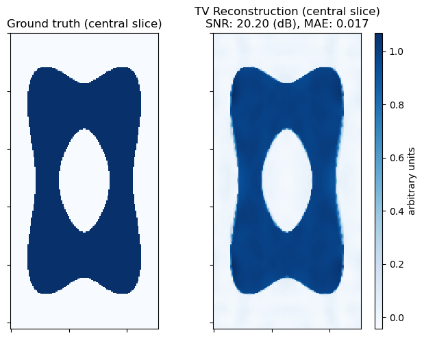
Show the recovered volume.
[5]:
fig, ax = kplt.subplots(nrows=1, ncols=2, sharex=True, sharey=True, figsize=(7, 6))
kplt.imview(
tangle[32],
title="Ground truth",
cmap=kplt.cm.viridis,
show_cbar=None,
ax=ax[0],
)
kplt.imview(
tangle_recon[32],
title="TV Reconstruction\nSNR: %.2f (dB), MAE: %.3f"
% (metric.snr(tangle, tangle_recon), metric.mae(tangle, tangle_recon)),
cmap=kplt.cm.viridis,
ax=ax[1],
)
divider = make_axes_locatable(ax[1])
cax = divider.append_axes("right", size="5%", pad=0.2)
fig.colorbar(ax[1].get_images()[0], cax=cax, label="arbitrary units")
fig.suptitle("Central slice on $z$ axis (axis 0)")
fig.tight_layout()
fig.show()
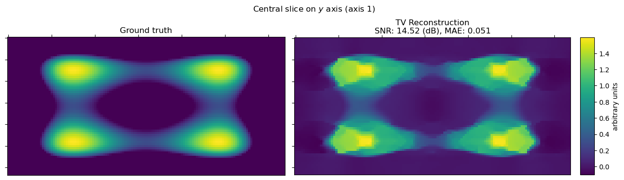
fig, ax = kplt.subplots(
nrows=1,
ncols=2,
sharex=True,
sharey=True,
gridspec_kw={"width_ratios": [1, 1.08]},
figsize=(13, 4),
)
kplt.imview(
tangle[:, 128],
title="Ground truth",
cmap=kplt.cm.viridis,
ax=ax[0],
)
kplt.imview(
tangle_recon[:, 128],
title="TV Reconstruction\nSNR: %.2f (dB), MAE: %.3f"
% (metric.snr(tangle, tangle_recon), metric.mae(tangle, tangle_recon)),
cmap=kplt.cm.viridis,
ax=ax[1],
)
divider = make_axes_locatable(ax[1])
cax = divider.append_axes("right", size="5%", pad=0.2)
fig.colorbar(ax[1].get_images()[0], ax=ax[1], cax=cax, label="arbitrary units")
fig.suptitle("Central slice on $y$ axis (axis 1)")
fig.tight_layout()
fig.show()