PPP (with BM4D) Volume Deconvolution
This example demonstrates the solution of a 3D image deconvolution problem (involving recovering a 3D volume that has been convolved with a 3D kernel and corrupted by noise) using the ADMM Plug-and-Play Priors (PPP) algorithm [56], with the BM4D [41] denoiser.
[1]:
import numpy as np

import komplot as kplt

import scico.numpy as snp
from scico import functional, linop, loss, metric, random
from scico.examples import create_3d_foam_phantom, downsample_volume, tile_volume_slices
from scico.optimize.admm import ADMM, LinearSubproblemSolver
from scico.util import device_info
kplt.config_notebook_plotting()
Create a ground truth image.
[2]:
np.random.seed(1234)
N = 128  # phantom size
Nx, Ny, Nz = N, N, N // 4
upsamp = 2
x_gt_hires = create_3d_foam_phantom((upsamp * Nz, upsamp * Ny, upsamp * Nx), N_sphere=100)
x_gt = downsample_volume(x_gt_hires, upsamp)
x_gt = snp.array(x_gt)  # convert to jax array
Set up forward operator and test signal consisting of blurred signal with additive Gaussian noise.
[3]:
n = 5  # convolution kernel size
σ = 20.0 / 255  # noise level

psf = snp.ones((n, n, n)) / (n**3)
A = linop.Convolve(h=psf, input_shape=x_gt.shape)

Ax = A(x_gt)  # blurred image
noise, key = random.randn(Ax.shape)
y = Ax + σ * noise
Set up ADMM solver.
[4]:
f = loss.SquaredL2Loss(y=y, A=A)
C = linop.Identity(x_gt.shape)

λ = 40.0 / 255  # BM4D regularization strength
g = λ * functional.BM4D()

ρ = 1.0  # ADMM penalty parameter
maxiter = 10  # number of ADMM iterations

solver = ADMM(
    f=f,
    g_list=[g],
    C_list=[C],
    rho_list=[ρ],
    x0=A.T @ y,
    maxiter=maxiter,
    subproblem_solver=LinearSubproblemSolver(cg_kwargs={"tol": 1e-3, "maxiter": 100}),
    itstat_options={"display": True},
)
Run the solver.
[5]:
print(f"Solving on {device_info()}\n")
x = solver.solve()
x = snp.clip(x, 0, 1)
hist = solver.itstat_object.history(transpose=True)
Solving on GPU (NVIDIA GeForce RTX 2080 Ti)

Iter  Time      Prml Rsdl  Dual Rsdl  CG It  CG Res
------------------------------------------------------
   0  1.49e+01  7.565e+00  2.582e+01      3  3.622e-04
   1  2.74e+01  3.812e+00  1.773e+01      3  3.765e-04
   2  3.77e+01  2.363e+00  1.264e+01      3  2.415e-04
   3  4.76e+01  1.793e+00  9.409e+00      2  9.223e-04
   4  5.75e+01  1.628e+00  7.278e+00      2  6.755e-04
   5  6.85e+01  1.581e+00  5.899e+00      2  5.100e-04
   6  7.89e+01  1.487e+00  4.893e+00      2  3.939e-04
   7  8.94e+01  1.397e+00  4.159e+00      2  3.069e-04
   8  9.91e+01  1.305e+00  3.610e+00      2  2.493e-04
   9  1.09e+02  1.255e+00  3.171e+00      2  2.148e-04
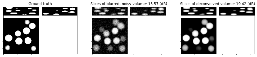
Show slices of the recovered 3D volume.
[6]:
show_id = Nz // 2
fig, ax = kplt.subplots(nrows=1, ncols=3, sharex=True, sharey=True, figsize=(15, 5))
kplt.imview(tile_volume_slices(x_gt), title="Ground truth", ax=ax[0])
nc = n // 2
yc = y[nc:-nc, nc:-nc, nc:-nc]
yc = snp.clip(yc, 0, 1)
kplt.imview(
    tile_volume_slices(yc),
    title="Slices of blurred, noisy volume: %.2f (dB)" % metric.psnr(x_gt, yc),
    ax=ax[1],
)
kplt.imview(
    tile_volume_slices(x),
    title="Slices of deconvolved volume: %.2f (dB)" % metric.psnr(x_gt, x),
    ax=ax[2],
)
fig.show()
Plot convergence statistics.
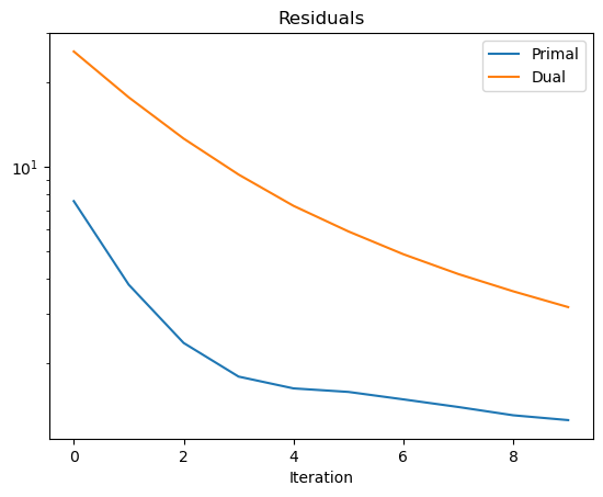
[7]:
kplt.plot(
    snp.array((hist.Prml_Rsdl, hist.Dual_Rsdl)).T,
    ylog=True,
    title="Residuals",
    xlabel="Iteration",
    legend=("Primal", "Dual"),
)
[7]:
<komplot.LinePlot at 0x7481dc4c59a0>