Denoising with Approximate Total Variation Proximal Operator
This example demonstrates use of approximations to the proximal operators of isotropic [35] and anisotropic [34] total variation norms for solving denoising problems using proximal algorithms.
[1]:
import komplot as kplt
import matplotlib
from xdesign import SiemensStar, discrete_phantom

import scico.numpy as snp
import scico.random
from scico import functional, linop, loss, metric
from scico.optimize import AcceleratedPGM
from scico.optimize.admm import ADMM, LinearSubproblemSolver
from scico.util import device_info
kplt.config_notebook_plotting()
Create a ground truth image.
[2]:
N = 256  # image size
phantom = SiemensStar(16)
x_gt = snp.pad(discrete_phantom(phantom, N - 16), 8)
x_gt = x_gt / x_gt.max()
Add noise to create a noisy test image.
[3]:
σ = 0.5  # noise standard deviation
noise, key = scico.random.randn(x_gt.shape, seed=0)
y = x_gt + σ * noise
Denoise with isotropic total variation, solved via ADMM.
[4]:
λ_iso = 1.0e0
f = loss.SquaredL2Loss(y=y)
g_iso = λ_iso * functional.L21Norm()
C = linop.FiniteDifference(input_shape=x_gt.shape, circular=True)

solver = ADMM(
    f=f,
    g_list=[g_iso],
    C_list=[C],
    rho_list=[1e1],
    x0=y,
    maxiter=200,
    subproblem_solver=LinearSubproblemSolver(cg_kwargs={"tol": 1e-4, "maxiter": 25}),
    itstat_options={"display": True, "period": 25},
)
print(f"Solving on {device_info()}\n")
x_iso = solver.solve()
print()
Solving on GPU (NVIDIA GeForce RTX 2080 Ti)

Iter  Time      Objective  Prml Rsdl  Dual Rsdl  CG It  CG Res
-----------------------------------------------------------------
   0  1.65e+00  5.196e+04  8.073e+01  5.247e+02      0  0.000e+00
  25  4.20e+00  1.122e+04  2.975e+00  3.349e+01     21  9.220e-05
  50  5.61e+00  1.118e+04  4.650e-01  2.053e+00     12  8.197e-05
  75  6.45e+00  1.118e+04  2.187e-01  6.625e-01      8  8.074e-05
 100  7.09e+00  1.118e+04  1.326e-01  2.681e-01      7  8.358e-05
 125  7.52e+00  1.118e+04  8.980e-02  1.324e-01      2  9.707e-05
 150  7.90e+00  1.119e+04  6.428e-02  7.647e-02      4  9.121e-05
 175  8.26e+00  1.119e+04  4.903e-02  5.165e-02      3  9.137e-05
 199  8.55e+00  1.119e+04  3.934e-02  3.701e-02      1  8.896e-05
Denoise with anisotropic total variation, solved via ADMM.
[5]:
# Tune the weight to give the same data fidelity as the isotropic case.
λ_aniso = 8.68e-1
g_aniso = λ_aniso * functional.L1Norm()

solver = ADMM(
    f=f,
    g_list=[g_aniso],
    C_list=[C],
    rho_list=[1e1],
    x0=y,
    maxiter=200,
    subproblem_solver=LinearSubproblemSolver(cg_kwargs={"tol": 1e-4, "maxiter": 25}),
    itstat_options={"display": True, "period": 25},
)
x_aniso = solver.solve()
print()
Iter  Time      Objective  Prml Rsdl  Dual Rsdl  CG It  CG Res
-----------------------------------------------------------------
   0  1.67e-01  5.626e+04  9.616e+01  6.111e+02      0  0.000e+00
  25  2.23e+00  1.125e+04  2.803e+00  2.874e+01     20  8.819e-05
  50  3.74e+00  1.122e+04  4.489e-01  3.038e+00     12  8.733e-05
  75  4.68e+00  1.122e+04  1.844e-01  1.212e+00      8  8.747e-05
 100  5.43e+00  1.122e+04  1.052e-01  5.770e-01      3  8.074e-05
 125  5.98e+00  1.122e+04  6.944e-02  3.061e-01      6  9.054e-05
 150  6.38e+00  1.122e+04  4.613e-02  1.784e-01      2  6.365e-05
 175  6.81e+00  1.122e+04  3.264e-02  9.793e-02      1  8.909e-05
 199  7.35e+00  1.122e+04  2.645e-02  3.759e-02      1  9.077e-05
Denoise with isotropic total variation, solved using an approximation of the TV norm proximal operator.
[6]:
h = λ_iso * functional.IsotropicTVNorm(circular=True, input_shape=y.shape)
solver = AcceleratedPGM(
    f=f, g=h, L0=1e3, x0=y, maxiter=500, itstat_options={"display": True, "period": 50}
)
x_iso_aprx = solver.solve()
print()
Iter  Time      Objective  L          Residual
-----------------------------------------------
   0  7.83e-01  5.821e+04  1.000e+03  5.254e-01
  50  1.38e+00  1.543e+04  1.000e+03  3.254e-01
 100  1.63e+00  1.140e+04  1.000e+03  8.952e-02
 150  1.84e+00  1.127e+04  1.000e+03  1.905e-02
 200  2.18e+00  1.125e+04  1.000e+03  6.708e-03
 250  2.40e+00  1.125e+04  1.000e+03  3.826e-03
 300  2.63e+00  1.124e+04  1.000e+03  2.248e-03
 350  2.83e+00  1.124e+04  1.000e+03  1.754e-03
 400  3.01e+00  1.124e+04  1.000e+03  1.112e-03
 450  3.27e+00  1.124e+04  1.000e+03  1.023e-03
 499  3.48e+00  1.124e+04  1.000e+03  6.762e-04
Denoise with anisotropic total variation, solved using an approximation of the TV norm proximal operator.
[7]:
h = λ_aniso * functional.AnisotropicTVNorm(circular=True, input_shape=y.shape)
solver = AcceleratedPGM(
    f=f, g=h, L0=1e3, x0=y, maxiter=500, itstat_options={"display": True, "period": 50}
)
x_aniso_aprx = solver.solve()
print()
Iter  Time      Objective  L          Residual
-----------------------------------------------
   0  6.24e-01  6.528e+04  1.000e+03  6.211e-01
  50  9.32e-01  1.528e+04  1.000e+03  3.716e-01
 100  1.10e+00  1.144e+04  1.000e+03  8.148e-02
 150  1.25e+00  1.133e+04  1.000e+03  1.622e-02
 200  1.45e+00  1.132e+04  1.000e+03  5.839e-03
 250  1.69e+00  1.132e+04  1.000e+03  3.472e-03
 300  1.90e+00  1.131e+04  1.000e+03  1.869e-03
 350  2.15e+00  1.132e+04  1.000e+03  1.550e-03
 400  2.40e+00  1.131e+04  1.000e+03  9.281e-04
 450  2.61e+00  1.131e+04  1.000e+03  9.358e-04
 499  2.80e+00  1.131e+04  1.000e+03  5.604e-04
Compute and print the data fidelity.
[8]:
for x, name in zip(
    (x_iso, x_aniso, x_iso_aprx, x_aniso_aprx),
    ("Isotropic", "Anisotropic", "Approx. Isotropic", "Approx. Anisotropic"),
):
    df = f(x)
    print(f"Data fidelity for {name} TV: {' ' * (20 - len(name))} {df:.2e}")
Data fidelity for Isotropic TV:             8.66e+03
Data fidelity for Anisotropic TV:           8.66e+03
Data fidelity for Approx. Isotropic TV:     8.65e+03
Data fidelity for Approx. Anisotropic TV:   8.66e+03
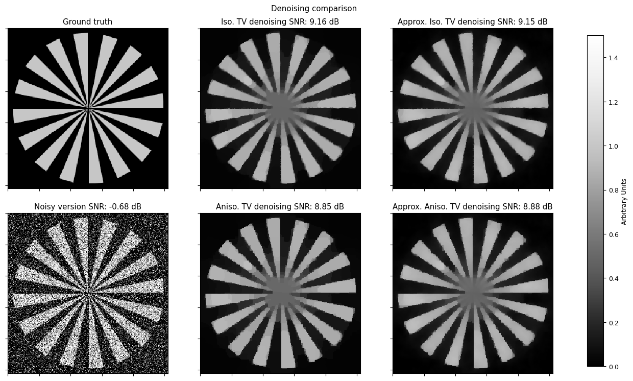
Plot results.
[9]:
matplotlib.rc("font", size=9)
plt_args = dict(norm=kplt.colors.Normalize(vmin=0, vmax=1.5))
fig, ax = kplt.subplots(nrows=2, ncols=3, sharex=True, sharey=True, figsize=(15, 8))
kplt.imview(x_gt, title="Ground truth", ax=ax[0, 0], **plt_args)
kplt.imview(
    y,
    title=f"Noisy version SNR: {metric.snr(x_gt, y):.2f} dB",
    ax=ax[1, 0],
    **plt_args,
)
kplt.imview(
    x_iso,
    title=f"Iso. TV denoising SNR: {metric.snr(x_gt, x_iso):.2f} dB",
    ax=ax[0, 1],
    **plt_args,
)
kplt.imview(
    x_aniso,
    title=f"Aniso. TV denoising SNR: {metric.snr(x_gt, x_aniso):.2f} dB",
    ax=ax[1, 1],
    **plt_args,
)
kplt.imview(
    x_iso_aprx,
    title=f"Approx. Iso. TV denoising SNR: {metric.snr(x_gt, x_iso_aprx):.2f} dB",
    ax=ax[0, 2],
    **plt_args,
)
kplt.imview(
    x_aniso_aprx,
    title=f"Approx. Aniso. TV denoising SNR: {metric.snr(x_gt, x_aniso_aprx):.2f} dB",
    ax=ax[1, 2],
    **plt_args,
)
fig.subplots_adjust(left=0.1, right=0.99, top=0.95, bottom=0.05, wspace=0.2, hspace=0.01)
fig.colorbar(
    ax[0, 0].get_images()[0], ax=ax, location="right", shrink=0.9, pad=0.05, label="Arbitrary Units"
)
fig.suptitle("Denoising comparison")
fig.show()