Video Decomposition via Robust PCA

This example demonstrates video foreground/background separation via a variant of the Robust PCA problem

\[\mathrm{argmin}_{\mathbf{x}_0, \mathbf{x}_1} \; (1/2) \| \mathbf{x}_0 + \mathbf{x}_1 - \mathbf{y} \|_2^2 + \lambda_0 \| \mathbf{x}_0 \|_* + \lambda_1 \| \mathbf{x}_1 \|_1 \;,\]

where \(\mathbf{x}_0\) and \(\mathbf{x}_1\) are respectively low-rank and sparse components, \(\| \cdot \|_*\) denotes the nuclear norm, and \(\| \cdot \|_1\) denotes the \(\ell_1\) norm.

Note: while video foreground/background separation is not an example of the scientific and computational imaging problems that are the focus of SCICO, it provides a convenient demonstration of Robust PCA, which does have potential application in scientific imaging problems.

import imageio.v3 as iio
import komplot as kplt

import scico.numpy as snp
from scico import functional, linop, loss
from scico.examples import rgb2gray
from scico.optimize.admm import ADMM, LinearSubproblemSolver
from scico.util import device_info
kplt.config_notebook_plotting()

Load example video.

vid = rgb2gray(
    iio.imread("imageio:newtonscradle.gif").transpose((1, 2, 3, 0)).astype(snp.float32) / 255.0
)

Construct matrix with each column consisting of a vectorised video frame.

y = vid.reshape((-1, vid.shape[-1]))

Define functional for Robust PCA problem.

A = linop.Sum(axis=0, input_shape=(2,) + y.shape)
f = loss.SquaredL2Loss(y=y, A=A)
C0 = linop.Slice(idx=0, input_shape=(2,) + y.shape)
g0 = functional.NuclearNorm()
C1 = linop.Slice(idx=1, input_shape=(2,) + y.shape)
g1 = functional.L1Norm()

Set up an ADMM solver object.

λ0 = 1e1  # nuclear norm regularization parameter
λ1 = 3e1  # ℓ1 norm regularization parameter
ρ0 = 2e1  # ADMM penalty parameter
ρ1 = 2e1  # ADMM penalty parameter
maxiter = 50  # number of ADMM iterations

solver = ADMM(
    f=f,
    g_list=[λ0 * g0, λ1 * g1],
    C_list=[C0, C1],
    rho_list=[ρ0, ρ1],
    x0=A.adj(y),
    maxiter=maxiter,
    subproblem_solver=LinearSubproblemSolver(),
    itstat_options={"display": True, "period": 10},
)

Run the solver.

print(f"Solving on {device_info()}\n")
x = solver.solve()
hist = solver.itstat_object.history(transpose=True)

Solving on GPU (NVIDIA GeForce RTX 2080 Ti)

Iter  Time      Objective  Prml Rsdl  Dual Rsdl  CG It  CG Res
-----------------------------------------------------------------
   0  3.15e+00  2.754e+05  3.429e+03  1.608e+04      1  5.520e-09
  10  4.85e+00  8.573e+03  1.059e+00  2.084e+01      1  6.830e-05
  20  5.10e+00  8.476e+03  1.088e-01  9.115e+00      1  2.762e-05
  30  5.33e+00  8.453e+03  6.044e-02  5.136e+00      1  1.536e-05
  40  5.56e+00  8.446e+03  3.353e-02  2.848e+00      1  8.519e-06
  49  5.76e+00  8.444e+03  2.166e-02  1.832e+00      1  5.502e-06

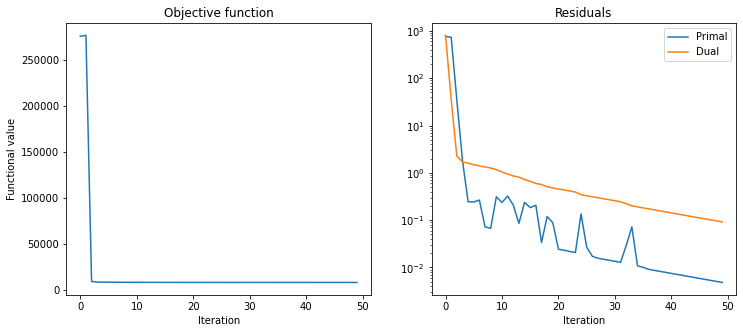
Plot convergence statistics.

fig, ax = kplt.subplots(nrows=1, ncols=2, figsize=(12, 5))
kplt.plot(
    hist.Objective,
    title="Objective function",
    xlabel="Iteration",
    ylabel="Functional value",
    ax=ax[0],
)
kplt.plot(
    snp.array((hist.Prml_Rsdl, hist.Dual_Rsdl)).T,
    ylog=True,
    title="Residuals",
    xlabel="Iteration",
    legend=("Primal", "Dual"),
    ax=ax[1],
)
fig.show()

Reshape low-rank component as background video sequence and sparse component as foreground video sequence.

xlr = C0(x)
xsp = C1(x)
vbg = xlr.reshape(vid.shape)
vfg = xsp.reshape(vid.shape)

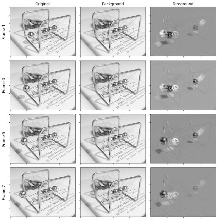
Display original video frames and corresponding background and foreground frames.

fig, ax = kplt.subplots(nrows=4, ncols=3, figsize=(10, 10))
ax[0][0].set_title("Original")
ax[0][1].set_title("Background")
ax[0][2].set_title("Foreground")
for n, fn in enumerate(range(1, 9, 2)):
    kplt.imview(vid[..., fn], ax=ax[n][0])
    kplt.imview(vbg[..., fn], ax=ax[n][1])
    kplt.imview(vfg[..., fn], ax=ax[n][2])
    ax[n][0].set_ylabel("Frame %d" % fn, labelpad=5, rotation=90, size="large")
fig.tight_layout()
fig.show()