Comparison of DnCNN Variants for Image Denoising

This example demonstrates the solution of an image denoising problem using DnCNN [64] networks trained for different noise levels, as well as custom variants with fewer network layers, and with a noise level input.

The networks trained for specific noise levels are labeled 6L, 6M, 6H, 17L, 17M, and 17H, where {6, 17} denote the number of layers, and {L, M, H} represent noise standard deviation of the training images (0.06, 0.10, and 0.20 respectively). The networks with a noise standard deviation input are labeled 6N and 17N, where {6, 17} again denote the number of layers.

import numpy as np

import komplot as kplt
from xdesign import Foam, discrete_phantom

import scico.numpy as snp
import scico.random
from scico import metric
from scico.denoiser import DnCNN
kplt.config_notebook_plotting()

Create a ground truth image.

np.random.seed(1234)
N = 512  # image size
x_gt = discrete_phantom(Foam(size_range=[0.075, 0.0025], gap=1e-3, porosity=1), size=N)
x_gt = snp.array(x_gt)  # convert to jax array

Test different DnCNN variants on images with different noise levels.

print("  σ   | variant | noisy image PSNR (dB)   | denoised image PSNR (dB)")
for σ in [0.06, 0.10, 0.20]:
    print("------+---------+-------------------------+-------------------------")
    for variant in ["17L", "17M", "17H", "17N", "6L", "6M", "6H", "6N"]:
        # Instantiate a DnCNN.
        denoiser = DnCNN(variant=variant)

        # Generate a noisy image.
        noise, key = scico.random.randn(x_gt.shape, seed=0)
        y = x_gt + σ * noise

        if variant in ["6N", "17N"]:
            x_hat = denoiser(y, sigma=σ)
        else:
            x_hat = denoiser(y)

        x_hat = np.clip(x_hat, a_min=0, a_max=1.0)

        if variant[0] == "6":
            variant += " "  # add spaces to maintain alignment

        print(
            " %.2f | %s     |          %.2f          |          %.2f          "
            % (σ, variant, metric.psnr(x_gt, y), metric.psnr(x_gt, x_hat))
        )

  σ   | variant | noisy image PSNR (dB)   | denoised image PSNR (dB)
------+---------+-------------------------+-------------------------
 0.06 | 17L     |          24.44          |          33.87
 0.06 | 17M     |          24.44          |          34.05
 0.06 | 17H     |          24.44          |          26.34
 0.06 | 17N     |          24.44          |          35.66
 0.06 | 6L      |          24.44          |          33.90
 0.06 | 6M      |          24.44          |          29.80
 0.06 | 6H      |          24.44          |          26.89
 0.06 | 6N      |          24.44          |          36.54
------+---------+-------------------------+-------------------------
 0.10 | 17L     |          20.01          |          27.46
 0.10 | 17M     |          20.01          |          31.96
 0.10 | 17H     |          20.01          |          26.48
 0.10 | 17N     |          20.01          |          30.37
 0.10 | 6L      |          20.01          |          27.93
 0.10 | 6M      |          20.01          |          27.50
 0.10 | 6H      |          20.01          |          26.58
 0.10 | 6N      |          20.01          |          33.36
------+---------+-------------------------+-------------------------
 0.20 | 17L     |          13.99          |          18.40
 0.20 | 17M     |          13.99          |          20.13
 0.20 | 17H     |          13.99          |          26.07
 0.20 | 17N     |          13.99          |          21.31
 0.20 | 6L      |          13.99          |          18.73
 0.20 | 6M      |          13.99          |          20.73
 0.20 | 6H      |          13.99          |          24.87
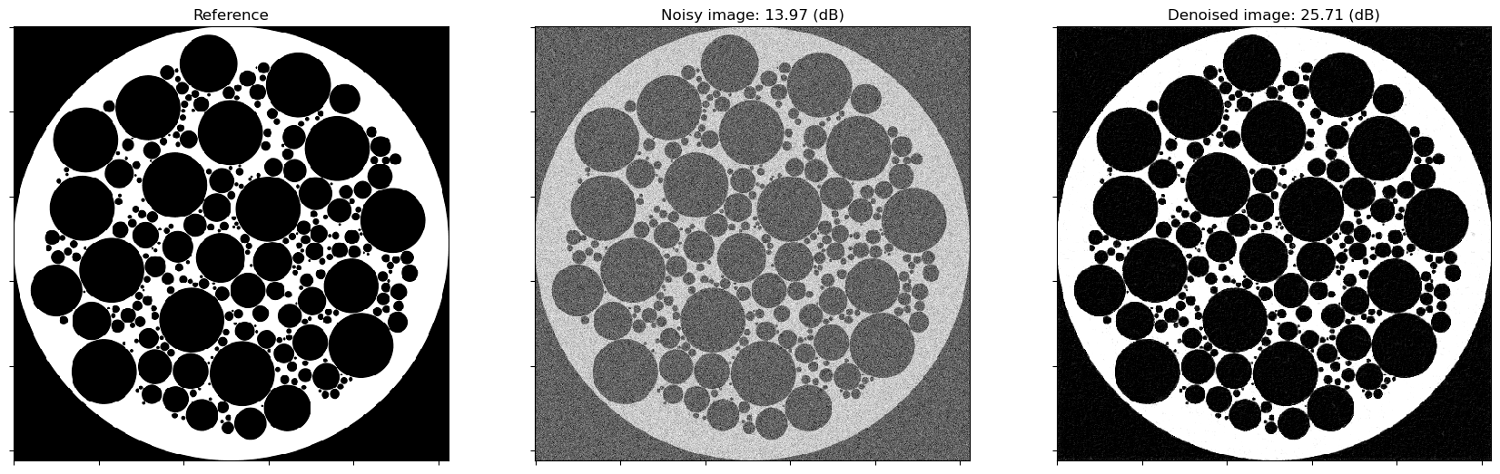
 0.20 | 6N      |          13.99          |          25.92

Show reference and denoised images for σ=0.2 and variant=6N.

fig, ax = kplt.subplots(nrows=1, ncols=3, sharex=True, sharey=True, figsize=(21, 7))
kplt.imview(x_gt, cmap="Blues", title="Reference", ax=ax[0])
kplt.imview(y, cmap="Blues", title="Noisy image: %.2f (dB)" % metric.psnr(x_gt, y), ax=ax[1])
kplt.imview(
    x_hat, cmap="Blues", title="Denoised image: %.2f (dB)" % metric.psnr(x_gt, x_hat), ax=ax[2]
)
fig.show()