3D TV-Regularized Sparse-View CT Reconstruction (Proximal ADMM Solver)
This example demonstrates solution of a sparse-view, 3D CT reconstruction problem with isotropic total variation (TV) regularization
where \(C\) is the X-ray transform (the CT forward projection operator), \(\mathbf{y}\) is the sinogram, \(D\) is a 3D finite difference operator, and \(\mathbf{x}\) is the desired image.
In this example the problem is solved via proximal ADMM, while standard ADMM is used in a companion example.
[1]:
import numpy as np

from mpl_toolkits.axes_grid1 import make_axes_locatable

import scico.numpy as snp
from scico import functional, linop, loss, metric, plot
from scico.examples import create_tangle_phantom
from scico.linop.xray.astra import XRayTransform3D, angle_to_vector
from scico.optimize import ProximalADMM
from scico.util import device_info
plot.config_notebook_plotting()
Create a ground truth image and projector.
[2]:
Nx = 128
Ny = 256
Nz = 64

tangle = snp.array(create_tangle_phantom(Nx, Ny, Nz))

n_projection = 10  # number of projections
angles = np.linspace(0, np.pi, n_projection)  # evenly spaced projection angles
det_spacing = [1.0, 1.0]
det_count = [Nz, max(Nx, Ny)]
vectors = angle_to_vector(det_spacing, angles)

# It would have been more straightforward to use the det_spacing and angles keywords
# in this case (since vectors is just computed directly from these two quantities), but
# the more general form is used here as a demonstration.
C = XRayTransform3D(tangle.shape, det_count=det_count, vectors=vectors)  # CT projection operator
y = C @ tangle  # sinogram
Set up problem and solver. We want to minimize the functional
where \(C\) is the convolution operator and \(D\) is a finite difference operator. This problem can be expressed as
which can be written in the form of a standard ADMM problem
with
This is a more complex splitting than that used in the companion example, but it allows the use of a proximal ADMM solver in a way that avoids the need for the conjugate gradient sub-iterations used by the ADMM solver in the companion example.
[3]:
𝛼 = 1e2  # improve problem conditioning by balancing C and D components of A
λ = 2e0 / 𝛼  # ℓ2,1 norm regularization parameter
ρ = 5e-3  # ADMM penalty parameter
maxiter = 1000  # number of ADMM iterations

f = functional.ZeroFunctional()
g0 = loss.SquaredL2Loss(y=y)
g1 = λ * functional.L21Norm()
g = functional.SeparableFunctional((g0, g1))
D = linop.FiniteDifference(input_shape=tangle.shape, append=0)

A = linop.VerticalStack((C, 𝛼 * D))
mu, nu = ProximalADMM.estimate_parameters(A)

solver = ProximalADMM(
    f=f,
    g=g,
    A=A,
    B=None,
    rho=ρ,
    mu=mu,
    nu=nu,
    maxiter=maxiter,
    itstat_options={"display": True, "period": 50},
)
Run the solver.
[4]:
print(f"Solving on {device_info()}\n")
tangle_recon = solver.solve()
hist = solver.itstat_object.history(transpose=True)

print(
    "TV Restruction\nSNR: %.2f (dB), MAE: %.3f"
    % (metric.snr(tangle, tangle_recon), metric.mae(tangle, tangle_recon))
)
Solving on GPU (NVIDIA GeForce RTX 2080 Ti)
Iter Time Objective Prml Rsdl Dual Rsdl
-----------------------------------------------
0 3.18e+00 1.438e+04 3.358e+04 3.358e+04
50 6.35e+00 3.979e+05 2.080e+04 3.847e+02
100 8.64e+00 3.262e+05 1.236e+04 3.351e+02
150 1.09e+01 2.910e+05 7.134e+03 2.676e+02
200 1.33e+01 2.323e+05 4.149e+03 1.960e+02
250 1.56e+01 2.152e+05 2.678e+03 1.547e+02
300 1.80e+01 1.950e+05 1.900e+03 1.216e+02
350 2.03e+01 1.876e+05 1.239e+03 1.011e+02
400 2.26e+01 1.796e+05 7.456e+02 7.383e+01
450 2.49e+01 1.740e+05 6.475e+02 5.413e+01
500 2.72e+01 1.707e+05 6.710e+02 4.320e+01
550 2.95e+01 1.699e+05 5.563e+02 3.627e+01
600 3.19e+01 1.670e+05 3.992e+02 2.929e+01
650 3.42e+01 1.665e+05 2.604e+02 2.339e+01
700 3.65e+01 1.667e+05 1.622e+02 2.019e+01
750 3.88e+01 1.652e+05 1.409e+02 1.623e+01
800 4.10e+01 1.658e+05 1.480e+02 1.514e+01
850 4.33e+01 1.649e+05 1.380e+02 1.324e+01
900 4.55e+01 1.651e+05 1.093e+02 1.142e+01
950 4.78e+01 1.649e+05 7.344e+01 9.757e+00
999 5.00e+01 1.648e+05 4.437e+01 8.498e+00
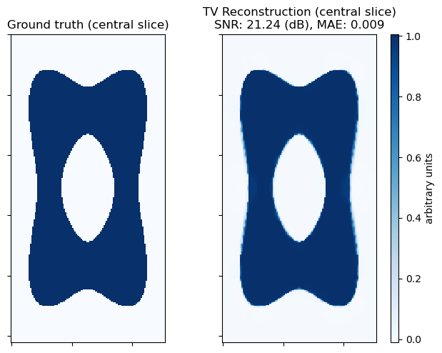
TV Restruction
SNR: 21.24 (dB), MAE: 0.009
Show the recovered image.
[5]:
fig, ax = plot.subplots(nrows=1, ncols=2, figsize=(7, 6))
plot.imview(
    tangle[32],
    title="Ground truth (central slice)",
    cmap=plot.cm.Blues,
    cbar=None,
    fig=fig,
    ax=ax[0],
)
plot.imview(
    tangle_recon[32],
    title="TV Reconstruction (central slice)\nSNR: %.2f (dB), MAE: %.3f"
    % (metric.snr(tangle, tangle_recon), metric.mae(tangle, tangle_recon)),
    cmap=plot.cm.Blues,
    fig=fig,
    ax=ax[1],
)
divider = make_axes_locatable(ax[1])
cax = divider.append_axes("right", size="5%", pad=0.2)
fig.colorbar(ax[1].get_images()[0], cax=cax, label="arbitrary units")
fig.show()